Deep Learning for Click Prediction in Mobile AdTech
Source: https://pixabay.com/illustrations/rays-stars-light-explosion-galaxy-9350519/Machine Learning for Real-Time BiddingThe past few years were a revolution for the mobile advertising and gaming industries, with the broad adoption of neural networks for advertising tasks, including click prediction. This migration occurred prior to the success of Large Language Models (LLMs) and other AI innovations, but is building on the momentum of this wave. The mobile gaming industry is spending billions on User Acquisition every year, and top players in this space such as Applovin have market caps of over $100B. In this post, we’ll discuss a conventional ML approach for click prediction, offer motivations for the migration to deep learning for this task, provide a hands-on example of the benefits of this approach using a data set from Kaggle, and detail some of the enhancements that this approach provides.Most large tech companies in the AdTech space are likely using deep learning for predicting user behavior. Social Media platforms have embraced the migration from classic machine learning (ML) to deep learning, as indicated by this Reddit post and this LinkedIn post. In the mobile gaming space Moloco, Liftoff, and Applovin have all shared details on their migration to deep learning or hardware acceleration to improve their user acquisition platforms. Most Demand Side Platforms (DSPs) are now looking to leverage neural networks to improve the value that their platforms provide for mobile user acquisition.We’ll start by discussing logistic regression as an industry standard for predicting user actions, discuss some of the shortfalls of this approach, and then showcase deep learning as a solution for click prediction. We’ll provide a deep dive on implementations for both a classic ML notebook and deep learning notebook for the task of predicting if a user is going to click on an ad. We won’t dive into the state of the art, but we will highlight where deep learning provides many benefits.All images in this post, with the exception of the header image, were created from by the author in the notebooks linked above. The Kaggle data set that we explore in this post has the CC0: Public Domain license.Cost Per Click ModelingOne of the goal types that DSPs typically provide for user acquisition is a cost per click model, where the advertiser is charged each time that the platform serves an impression on a mobile device and the user clicks. We’ll focus on this goal type to keep things simple, but most advertisers prefer goal types focused on driving installs or acquiring users that will spend money in their app.In programmatic bidding, a DSP is integrated with one or more ad exchanges, which provide inventory for the platform to bid on. Most exchanges use a version of the OpenRTB specification to send bid requests to DSPs and get back responses in a standardized format. For each ad request from a Supply Side Platform (SSP), the exchange runs an auction and the DSP that responds with the highest price wins. The exchange then provides the winning bid response to the SSP, which may result in an ad impression on a mobile device.In order for a DSP to integrate with an ad exchange, there is an onboarding process to make sure that the DSP can meet the technical requirements of an exchange, which typically requires DSPs to respond to bid requests within 120 milliseconds. What makes this a huge challenge is that some exchanges provide over 1 million bid requests per second, and DSPs are usually integrating with several exchanges. For example, Moloco responds to over 5 million requests per second (QPS) during peak capacity. Because of the latency requirements and massive scale of requests, it’s challenging to use machine learning for user acquisition within a DSP, but it’s also a requirement in order to meet advertiser goals.In order to make money as a DSP you need to be able to deliver ad impressions that meet your advertiser goals, while also generating net revenue. To accomplish this, a DSP needs to bid less than the expected value that an impression will deliver, while also bidding high enough to exceed the bid floor of a request and win in auctions against other DSPs. A demand-side platform is billed per impression shown, which corresponds to a CPM (cost per impression) model. If the advertiser goal is a target cost per click (CPC), then the DSP needs to translate the CPC value to a CPM value for bidding. We can do this using machine learning and predicting the likelihood of a user to click on an impression, which we call p_ctr. We can this calculate a bid price as follows:cpm = target_cpc * p_ctrbid_price = cpm * bid_shadeWe use the likelihood of a click event to convert from cost per click to cost per impression and then apply a bid shade with a value of less than 1.0 to make sure that we are delivering more value for advertisers than we are paying to the ad exchange for serving the impression.In order for a click prediction mode


Machine Learning for Real-Time Bidding
The past few years were a revolution for the mobile advertising and gaming industries, with the broad adoption of neural networks for advertising tasks, including click prediction. This migration occurred prior to the success of Large Language Models (LLMs) and other AI innovations, but is building on the momentum of this wave. The mobile gaming industry is spending billions on User Acquisition every year, and top players in this space such as Applovin have market caps of over $100B. In this post, we’ll discuss a conventional ML approach for click prediction, offer motivations for the migration to deep learning for this task, provide a hands-on example of the benefits of this approach using a data set from Kaggle, and detail some of the enhancements that this approach provides.
Most large tech companies in the AdTech space are likely using deep learning for predicting user behavior. Social Media platforms have embraced the migration from classic machine learning (ML) to deep learning, as indicated by this Reddit post and this LinkedIn post. In the mobile gaming space Moloco, Liftoff, and Applovin have all shared details on their migration to deep learning or hardware acceleration to improve their user acquisition platforms. Most Demand Side Platforms (DSPs) are now looking to leverage neural networks to improve the value that their platforms provide for mobile user acquisition.
We’ll start by discussing logistic regression as an industry standard for predicting user actions, discuss some of the shortfalls of this approach, and then showcase deep learning as a solution for click prediction. We’ll provide a deep dive on implementations for both a classic ML notebook and deep learning notebook for the task of predicting if a user is going to click on an ad. We won’t dive into the state of the art, but we will highlight where deep learning provides many benefits.
All images in this post, with the exception of the header image, were created from by the author in the notebooks linked above. The Kaggle data set that we explore in this post has the CC0: Public Domain license.
Cost Per Click Modeling
One of the goal types that DSPs typically provide for user acquisition is a cost per click model, where the advertiser is charged each time that the platform serves an impression on a mobile device and the user clicks. We’ll focus on this goal type to keep things simple, but most advertisers prefer goal types focused on driving installs or acquiring users that will spend money in their app.
In programmatic bidding, a DSP is integrated with one or more ad exchanges, which provide inventory for the platform to bid on. Most exchanges use a version of the OpenRTB specification to send bid requests to DSPs and get back responses in a standardized format. For each ad request from a Supply Side Platform (SSP), the exchange runs an auction and the DSP that responds with the highest price wins. The exchange then provides the winning bid response to the SSP, which may result in an ad impression on a mobile device.
In order for a DSP to integrate with an ad exchange, there is an onboarding process to make sure that the DSP can meet the technical requirements of an exchange, which typically requires DSPs to respond to bid requests within 120 milliseconds. What makes this a huge challenge is that some exchanges provide over 1 million bid requests per second, and DSPs are usually integrating with several exchanges. For example, Moloco responds to over 5 million requests per second (QPS) during peak capacity. Because of the latency requirements and massive scale of requests, it’s challenging to use machine learning for user acquisition within a DSP, but it’s also a requirement in order to meet advertiser goals.
In order to make money as a DSP you need to be able to deliver ad impressions that meet your advertiser goals, while also generating net revenue. To accomplish this, a DSP needs to bid less than the expected value that an impression will deliver, while also bidding high enough to exceed the bid floor of a request and win in auctions against other DSPs. A demand-side platform is billed per impression shown, which corresponds to a CPM (cost per impression) model. If the advertiser goal is a target cost per click (CPC), then the DSP needs to translate the CPC value to a CPM value for bidding. We can do this using machine learning and predicting the likelihood of a user to click on an impression, which we call p_ctr. We can this calculate a bid price as follows:
cpm = target_cpc * p_ctr
bid_price = cpm * bid_shade
We use the likelihood of a click event to convert from cost per click to cost per impression and then apply a bid shade with a value of less than 1.0 to make sure that we are delivering more value for advertisers than we are paying to the ad exchange for serving the impression.
In order for a click prediction model to perform well for programmatic user acquisition, we want a model that has the following properties:
- Large Bias
We want a click model that is highly discriminative and able to differentiate between impressions unlikely to result in a click and ones that are highly likely to result in a click. If a model does not have sufficient bias, it won’t be able to compete with other DSPs in auctions. - Well Calibrated
We want the predicted and actual conversion rates of the model to align well for the ad impressions the DSP purchases. This means we have a preference for models where the output can be interpreted as a probability of a conversion occurring. Poor calibration will result in inefficient spending. A sample calibration plot is shown below. - Fast Evaluation
We want to reduce our compute cost when bidding on millions of requests per second and have models that are fast to inference. - Parallel Evaluation
Ideally, we want to be able to run model inference in parallel to improve throughput. For a single bid request, a DSP may be considering hundreds of campaigns to bid for, and each one needs a p_ctr value.
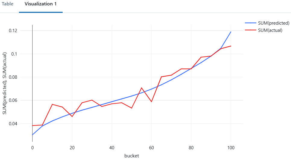
Many ad tech platforms started with logistic regression for click prediction, because they work well for the first 3 desired properties. Over time, it was discovered that deep learning models could perform better than logistic regression on the bias goal, with neural networks being better at discriminating between click and no-click impressions. Additionally, neural networks can use batch evaluation and align will with the fourth property of parallel evaluation.
DSPs were able to push logistic regression models pretty far, which is what we’ll cover in the next section, but they do have some boundaries in their application to user acquisition. Deep neural networks (DNN) can overcome some of these issues, but present new challenges of their own.
The Big Logistic Era
Ad Tech companies have been using logistic regression for more than a decade for click prediction. For example, Facebook presented using logit in combination with other models at ADKDD 2014. There are many different ways of using logistic regression for click prediction, but I’ll focus on a single approach I worked on in the past called Big Logistic. The general idea was to turn all of your features into tokens, create combinations of tokens to represent crosses or feature interactions, and then create a list of tokens that you use to convert your input features into a sparse vector representation. It’s an approach where every feature is 1-hot encoded and all of the features are binary, which helps simplify hyperparameter tuning for the click model. It’s an approach that can support numeric, categorical, and many-hot features as inputs.
To determine what this approach looks like in practice, we’ll provide a hands-on example of training a click prediction model using the CTR In Advertisement Kaggle data set. The full notebook for feature encoding, model training and evaluation is available here. I used Databricks, PySpark, and MLlib for this pipeline.
The dataset provides a training data set with labels and a test data set without labels. For this exercise we’ll split the training file into train and test groups, so that we have labels available for all records. We create a 90/10% split where the train set has 414k records and test has 46k records. The data set has 15 columns, which includes a label, 2 columns that we’ll ignore (session_id and user_id) and 12 categorical values that we’ll use as features in our model. A few sample records are shown in the table above.
The first step we’ll perform is tokenizing the data set, which is a form of 1-hot encoding. We convert each column to a string value by concatenating the feature name and feature value. For example, we would create the following tokens for the first row in the above table:
[“product_c”, “campaign_id_359520”, “webpage_id_13787”, ..]
For null values, we use “null” as the value, e.g. “product_null”. We also create all combinations of two features, which generates additional tokens:
[“product_c*campaign_id_359520”, “”, “product_c*webpage_id_13787”, “campaign_id_359520*webpage_id_13787”,..]
We use a UDF on the PySpark dataframe to convert the 12 columns into a vector of strings. The resulting dataframe includes the token list and label, as shown below.
We then create a top tokens list, assign an index to each token in this list, and use the mapping of token name to token index to encode the data. We limited our token list to values where we have at least 1000 examples, which resulted in roughly 2,500 tokens.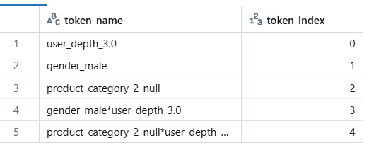
We then apply this token list to each record in the data set to convert from the token list to a sparse vector representation. If a record includes the token for an index, the value is set to 1, and if the token is missing the value is set to 0. This results in a data set that we can use with MLlib to train a logistic regression model.
We split the dataset into train and test groups, fit the model on the train data set, and then transform the test data set to get predictions.
classifier = LogisticRegression(featuresCol = 'features',\
    labelCol = 'label', maxIter = 50, regParam = 0.01, elasticNetParam = 0)
lr_model = classifier.fit(train_df)
pred_df = lr_model.transform(test_df).cache()
This process resulted in the following offline metrics, which we’ll compare to a deep learning model in the next section.
Actual Conv: 0.06890
Predicted Conv: 0.06770
Log Loss: 0.24795
ROC AUC: 0.58808
PR AUC: 0.09054
The AUC metrics don’t look great, but there isn’t much signal in the data set with the features that we explored, and other participants in the Kaggle competition generally had lower ROC metrics. One other limitation of the data set is that the categorical values are low cardinality, with only a small number of distinct values. This resulted in a low parameter count, with only 2,500 features, which limited the bias of the model.
Logistic regression works great for click prediction, but where we run into challenges is when dealing with high cardinality features. In mobile ad tech, the publisher app, where the ad is rendered, is a high cardinality feature, because there are millions of potential mobile apps that may render an ad. If we want to include the publisher app as a feature in our model, and are using 1-hot encoding, we are going to end up with a large parameter count. This is especially the case when we perform feature crosses between the publisher app and other high cardinality features, such as the device model.
I’ve worked with logistic regression click models that have more than 50 million parameters. At this scale, MLlib’s implementation of logistic regression runs into training issues, because it densifies the vectors in its training loop. To avoid this bottleneck, I used the Fregata library, which performs gradient descent using the sparse vector directly in a model averaging strategy.
The other issue with large click models is model inference. If you include too many parameters in your logit model, it may be slow to evaluate, significantly increasing your model serving costs.
The Deep Learning Era
Deep learning is a good solution for click models, because it provides methods for working efficiently with very sparse features with high cardinality. One of the key layers that we’ll use in our deep learning model is an embedding layer, which takes a categorical feature as an input and a dense vector as an output. With an embedding layer, we learn a vector for each of the entries in our vocabulary for a categorical feature, and the number of parameters is the size of the vocabulary times the output dense vector size, which we can control. Neural networks can reduce the parameter count by creating interactions between the dense layers output of embeddings, rather than making crosses between the sparse 1-hot encoded approach used in logistic regression.
Embedding layers are just one way that neural networks can provide improvements over logistic regression models, because deep learning frameworks provide a variety of layer types and architectures. We’ll focus on embeddings for our sample model to keep things simplistic. We’ll create a pipeline for encoding the data set into TensorFlow Records and then train a model using embeddings and cross layers to perform click prediction. The full notebook for data preparation, model training and evaluation is available here.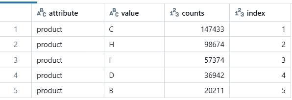
The first step that we perform is generating a vocabulary for each of the features that we want to encode. For each feature, we find all values with more than 100 instances, and everything else is grouped into an out-of-vocab (OOV) value. We then encode all of the categorical features and combine them into a single tensor named int, as shown below.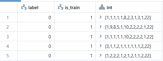
We then save the Spark dataframe as TensorFlow records to cloud storage.
output_path = "dbfs:/mnt/ben/kaggle/train/"
train_df.write.format("tfrecords").mode("overwrite").save(output_path)
We then copy the files to the driver node and create TensorFlow data sets for training and evaluating the model.
def getRecords(paths):
    features = {
        'int': FixedLenFeature([len(vocab_sizes)], tf.int64),
        'label': FixedLenFeature([1], tf.int64)
    }

    @tf.function
    def _parse_example(x):
        f = tf.io.parse_example(x, features)
        return f, f.pop("label")

    dataset = tf.data.TFRecordDataset(paths)
    dataset = dataset.batch(10000)
    dataset = dataset.map(_parse_example)
    return dataset

training_data = getRecords(train_paths)
test_data = getRecords(test_paths)
We then create a Keras model, where the input layer is an embedding layer per categorical feature, we have two hidden cross layers, and a final output layer that is a sigmoid activation for the propensity prediction.
cat_input = tf.keras.Input(shape=(len(vocab_sizes)),\
    name = "int", dtype='int64')
input_layers = [cat_input]

cross_inputs = []
for attribute in categories_index:
    index = categories_index[attribute]
    size = vocab_sizes[attribute]

    category_input = cat_input[:,(index):(index+1)]
    embedding = keras.layers.Flatten()\
        (keras.layers.Embedding(size, 5)(category_input))
    cross_inputs.append(embedding)

cross_input = keras.layers.Concatenate()(cross_inputs)
cross_layer = tfrs.layers.dcn.Cross()
crossed_ouput = cross_layer(cross_input, cross_input)

cross_layer = tfrs.layers.dcn.Cross()
crossed_ouput = cross_layer(cross_input, crossed_ouput)

sigmoid_output=tf.keras.layers.Dense(1,activation="sigmoid")(crossed_ouput)
model = tf.keras.Model(inputs=input_layers, outputs = [ sigmoid_output ])
model.summary()
The resulting model has 7,951 parameters, which is about 3 times the size of our logistic regression model. If the categories had larger cardinalities, then we would expect the parameter count of the logit model to be higher. We train the model for 40 epochs:
metrics=[tf.keras.metrics.AUC(), tf.keras.metrics.AUC(curve="PR")]

model.compile(optimizer=tf.keras.optimizers.Adam(learning_rate=1e-3),\
    loss=tf.keras.losses.BinaryCrossentropy(), metrics=metrics)
history = model.fit(x = training_data, epochs = 40,\
    validation_data = test_data, verbose=0)
We can now compare the offline metrics between our logistic regression and DNN models:
                Logit    DNN
Actual Conv:    0.06890  0.06890
Predicted Conv: 0.06770  0.06574
Log Loss:       0.24795  0.24758
ROC AUC:        0.58808  0.59284
PR AUC:         0.09054  0.09249
We do see improvements to the log loss metric where lower is better and the AUC metrics where higher is better. The main improvement is to the precision-recall (PR) AUC metric, which may help the model perform better in auctions. One of the issues with the DNN model is that the model calibration is worse, and the DNN average predicted value is further off than the logistic regression model. We would need to do a bit more model tuning to improve the calibration of the model.
What’s Next?
We are now in the era of deep learning for ad tech and companies are using a variety of architectures to deliver advertiser goals for user acquisition. In this post, we showed how migrating from logistic regression to a simple neural network with embedding layers can provide better offline metrics for a click prediction model. Here are some additional ways we could leverage deep learning to improve click prediction:
- Use Embeddings from Pre-trained Models
We can use models such as BERT to convert app store descriptions into vectors that we can use as input to the click model. - Explore New Architectures
We could explore the DCN and TabTransformer architectures. - Add Non-Tabular Data
We could use img2vec to create input embeddings from creative assets.
Thanks for reading!
Ben Weber is a machine learning engineer with over a decade of experience in gaming and ad tech with prior roles at Zynga, Microsoft, Amazon, and Electronic Arts.
Deep Learning for Click Prediction in Mobile AdTech was originally published in Towards Data Science on Medium, where people are continuing the conversation by highlighting and responding to this story.
What's Your Reaction?









_Elena_Uve_Alamy.jpg?#)


.png?width=1920&height=1920&fit=bounds&quality=80&format=jpg&auto=webp#)

