Static and Dynamic Attention: Implications for Graph Neural Networks
Examining the expressive capacity of Graph Attention NetworksImage by the authorIn graph representation learning, neighborhood aggregation is one of the most well-studied and investigated areas, among which attention-based methods largely remain state-of-the-art. Leveraging learnable attention scores for weighted aggregations, graph attention networks exhibit higher expressivity than naive aggregation schemes. In graph attention, the most well known and used schemes are from Graph Attention Networks (GAT) [1] and How Attentive are Graph Attention Networks (GATv2) [2]. GAT and GATv2 both leverage attention for weighted neighborhood aggregation, but differ in how they employ attention scores, resulting in differing levels of theoretical expressivity. The chief purpose of this article is to explore exactly how GAT and GATv2 differ in their formulations and why it results in different levels of expressive capacity.Graph Attention Network (GAT)Graph Attention Network (GAT), as introduced in [1], closely follows the work from [3] in its attention setup. GAT formulation also holds many similarities to the now infamous transformer paper [4], with both papers having been published months away from each other.Attention in graphs is used to rank or weigh the relative importance of every neighboring node (keys) with respect to each source node (query). These attention scores are calculated for every node feature in the graph and its respective neighbors. Node features, denoted bygo through a linear transformation with a weight matrix denotedbefore attention mechanism is applied. With linearly transformed node features, raw attention score is calculated as shown in Equation (1). To calculate normalized attention scores, softmax function is used as shown in Equation (2) similar to attention calculation in [4].In the paper (GAT), the attention mechanism Attention( ) used is a single-layer feedforward neural network parameterized by a followed by a LeakyReLU non-linearity, as shown in Equation (3). The || symbol denotes concatenation along the feature dimension. Note: multi-head attention formulation is intentionally skipped in this article as it holds no relevance to attention formulation itself. Both GAT and GATv2 leverage multi-headed attention in their implementations.As it can be seen, the learnable attention parameter a is introduced as a linear combination to the transformed node features Wh. As elaborated in the upcoming sections, this setup is known as static attention and is the main limiting factor of GAT, though for reasons that are not immediately obvious.Static AttentionConsider the following graph below where node h1 is the query node with the following neighbors (keys) {h2, h3, h4, h5}.Image by the authorCalculating the raw attention score between the query node and h2 following the GAT formulation is shown in Equation (4).As mentioned earlier, learnable attention parameter a is combined linearly with the concatenated query and key nodes. This means that the contributions of a with respect to Wh1 and Wh2 are linearly separable as a = [a1 || a2]. Using a1 and a2, Equation (4) can be restructured as the following (Equation (5)).Calculating the raw attention scores for the rest of the neighborhood with respect to the query node h1, a pattern begins to emerge.From Equation (6), it can be seen that the query termis repeated each time in the calculation of attention scores e. This means that while the query term is technically included in the attention calculation, it essentially affects all neighbors equally and does not affect their relative ordering. Only the key termsdetermine the relative order of attention scores with respect to each other.This type of attention is called static attention by [2]. This design means that the ranking of neighbors’ importanceis determined globally across all nodes independent of the specific query nodes. This limitation prevents GAT from capturing locally nuanced relationships where different nodes might prioritize different subsets of neighbors. As stated in [2], “[static attention] cannot model situations where different keys have different relevance to different queries”.Dynamic Attention and GATv2Authors of GATv2 make the observation that application of consecutive, linear operations on W, and a (as in Equation (4)) can be collapsed into a single linear layer. Indeed, the attention scores being unconditioned on the query terms is a byproduct of such linear operations between W, H, and a. To overcome such limitations of static attention, GATv2 introduces what they call dynamic attention that removes above-mentioned linearity constraint and makes attention scores conditional on their query nodes, allowing for a strictly more expressive attention mechanism.Dynamic attention is achieved with a simple change in the order of operations in GAT’s attention calculation process. This simple change essentially amounts to applying the non-linearity to query and key terms before introdu
Examining the expressive capacity of Graph Attention Networks

In graph representation learning, neighborhood aggregation is one of the most well-studied and investigated areas, among which attention-based methods largely remain state-of-the-art. Leveraging learnable attention scores for weighted aggregations, graph attention networks exhibit higher expressivity than naive aggregation schemes. In graph attention, the most well known and used schemes are from Graph Attention Networks (GAT) [1] and How Attentive are Graph Attention Networks (GATv2) [2]. GAT and GATv2 both leverage attention for weighted neighborhood aggregation, but differ in how they employ attention scores, resulting in differing levels of theoretical expressivity. The chief purpose of this article is to explore exactly how GAT and GATv2 differ in their formulations and why it results in different levels of expressive capacity.
Graph Attention Network (GAT)
Graph Attention Network (GAT), as introduced in [1], closely follows the work from [3] in its attention setup. GAT formulation also holds many similarities to the now infamous transformer paper [4], with both papers having been published months away from each other.
Attention in graphs is used to rank or weigh the relative importance of every neighboring node (keys) with respect to each source node (query). These attention scores are calculated for every node feature in the graph and its respective neighbors. Node features, denoted by
go through a linear transformation with a weight matrix denoted
before attention mechanism is applied. With linearly transformed node features, raw attention score is calculated as shown in Equation (1). To calculate normalized attention scores, softmax function is used as shown in Equation (2) similar to attention calculation in [4].
In the paper (GAT), the attention mechanism Attention( ) used is a single-layer feedforward neural network parameterized by a followed by a LeakyReLU non-linearity, as shown in Equation (3). The || symbol denotes concatenation along the feature dimension. Note: multi-head attention formulation is intentionally skipped in this article as it holds no relevance to attention formulation itself. Both GAT and GATv2 leverage multi-headed attention in their implementations.

As it can be seen, the learnable attention parameter a is introduced as a linear combination to the transformed node features Wh. As elaborated in the upcoming sections, this setup is known as static attention and is the main limiting factor of GAT, though for reasons that are not immediately obvious.
Static Attention
Consider the following graph below where node h1 is the query node with the following neighbors (keys) {h2, h3, h4, h5}.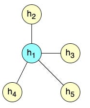
Calculating the raw attention score between the query node and h2 following the GAT formulation is shown in Equation (4).
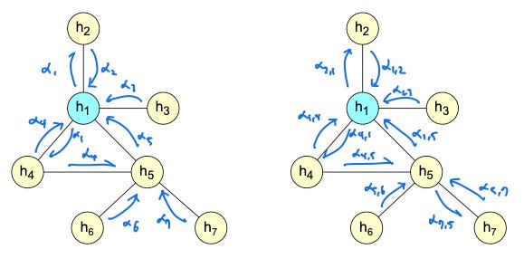
As mentioned earlier, learnable attention parameter a is combined linearly with the concatenated query and key nodes. This means that the contributions of a with respect to Wh1 and Wh2 are linearly separable as a = [a1 || a2]. Using a1 and a2, Equation (4) can be restructured as the following (Equation (5)).
Calculating the raw attention scores for the rest of the neighborhood with respect to the query node h1, a pattern begins to emerge.
From Equation (6), it can be seen that the query term
is repeated each time in the calculation of attention scores e. This means that while the query term is technically included in the attention calculation, it essentially affects all neighbors equally and does not affect their relative ordering. Only the key terms
determine the relative order of attention scores with respect to each other.
This type of attention is called static attention by [2]. This design means that the ranking of neighbors’ importance
is determined globally across all nodes independent of the specific query nodes. This limitation prevents GAT from capturing locally nuanced relationships where different nodes might prioritize different subsets of neighbors. As stated in [2], “[static attention] cannot model situations where different keys have different relevance to different queries”.
Dynamic Attention and GATv2
Authors of GATv2 make the observation that application of consecutive, linear operations on W, and a (as in Equation (4)) can be collapsed into a single linear layer. Indeed, the attention scores being unconditioned on the query terms is a byproduct of such linear operations between W, H, and a. To overcome such limitations of static attention, GATv2 introduces what they call dynamic attention that removes above-mentioned linearity constraint and makes attention scores conditional on their query nodes, allowing for a strictly more expressive attention mechanism.
Dynamic attention is achieved with a simple change in the order of operations in GAT’s attention calculation process. This simple change essentially amounts to applying the non-linearity to query and key terms before introducing the a layer, as demonstrated in Equation (7).
While simple and intuitive, this tweak in the order of operations means that the query and key terms are no longer linearly separable. It also means that when the attention mechanism is applied, both the query and key terms interact with a in a way that allows attention scores to be conditioned on both the query and its neighbors. As simple as this change may look, it represents a deep idea in attention mechanism and makes significant progress in the theoretical expressive capacity that graph attention can introduce to a problem.
Final Thoughts
While GATv2 undoubtedly makes significant progress over GAT in their use of attention mechanism, such progress is largely theoretical. While the authors of GATv2 do devise benchmark scenarios that clearly illustrate the expressive power of dynamic attention and the shortcomings of static attention, GAT still shows competitive performance in many existing real-world problems and datasets. In fact, GATv2 only shows very marginal improvements in performance against GAT in nearly all of the real-world datasets used in their experimentation (including in various OGB datasets and QM9 dataset).
The juxtaposition between GATv2’s significant theoretical advancement and its marginal empirical improvement can be due to several factors. One, conditioned on the query or not, attention mechanism has been shown to be very effective and can present stable and powerful performance especially under multi-headed settings. Two, the scenarios that would most benefit from GATv2’s dynamic attention formulation may not arise all that much in real world graphs. GATv2’s dynamic attention would be most beneficial in graphs exhibiting complex local interactions between nodes requiring different nodes to have distinctly different rankings of (possibly) shared neighbors. It may be the case that such graphs are simply not common or realistic. In homophilic graphs for example, keys that rank highly according to a particular query may very well be of global importance and likely of high importance among other local queries. In addition, real-world graphs can often be sparse with relatively low average degrees. With such graphs, the benefits of dynamic attention may be less pronounced because there are fewer neighbors to rank dynamically.
Overall, both GAT and GATv2 are among the most versatile, powerful, and practically used operations in graph representation learning. I want to highlight 2 things to sum up this article:
- Despite the name “v2”, GATv2 is more than just an iterative update or optimization of GAT and offers real theoretical improvements to its predecessor.
- Not only has GAT been incredibly influential since its introduction in 2018, it still remains one of the most powerful tools available in graph representation learning.
My code implementation on Github: https://github.com/timlee0131/graph-attention-networks
References
[1] Petar Veliˇckovi´c, Guillem Cucurull, Arantxa Casanova, Adriana Romero, Pietro Lio, and Yoshua Bengio. Graph attention networks. arXiv preprint arXiv:1710.10903, 2017.
[2] Shaked Brody, Uri Alon, and Eran Yahav. How attentive are graph attention networks? arXiv preprint arXiv:2105.14491, 2021.
[3] Dzmitry Bahdanau. Neural machine translation by jointly learning to align and translate. arXiv preprint arXiv:1409.0473, 2014.
[4] A Vaswani. Attention is all you need. Advances in Neural Information Processing Systems, 2017.
Static and Dynamic Attention: Implications for Graph Neural Networks was originally published in Towards Data Science on Medium, where people are continuing the conversation by highlighting and responding to this story.


