Neural Networks – Intuitively and Exhaustively Explained

An in-depth exploration of the most fundamental architecture in modern AI

In this article we’ll form a thorough understanding of the neural network, a cornerstone technology underpinning virtually all cutting edge AI systems. We’ll first explore neurons in the human brain, and then explore how they formed the fundamental inspiration for neural networks in AI. We’ll then explore back-propagation, the algorithm used to train neural networks to do cool stuff. Finally, after forging a thorough conceptual understanding, we’ll implement a Neural Network ourselves from scratch and train it to solve a toy problem.

Who is this useful for? Anyone who wants to form a complete understanding of the state of the art of AI.

How advanced is this post? This article is designed to be accessible to beginners, and also contains thorough information which may serve as a useful refresher for more experienced readers.

Pre-requisites: None

Inspiration From the Brain

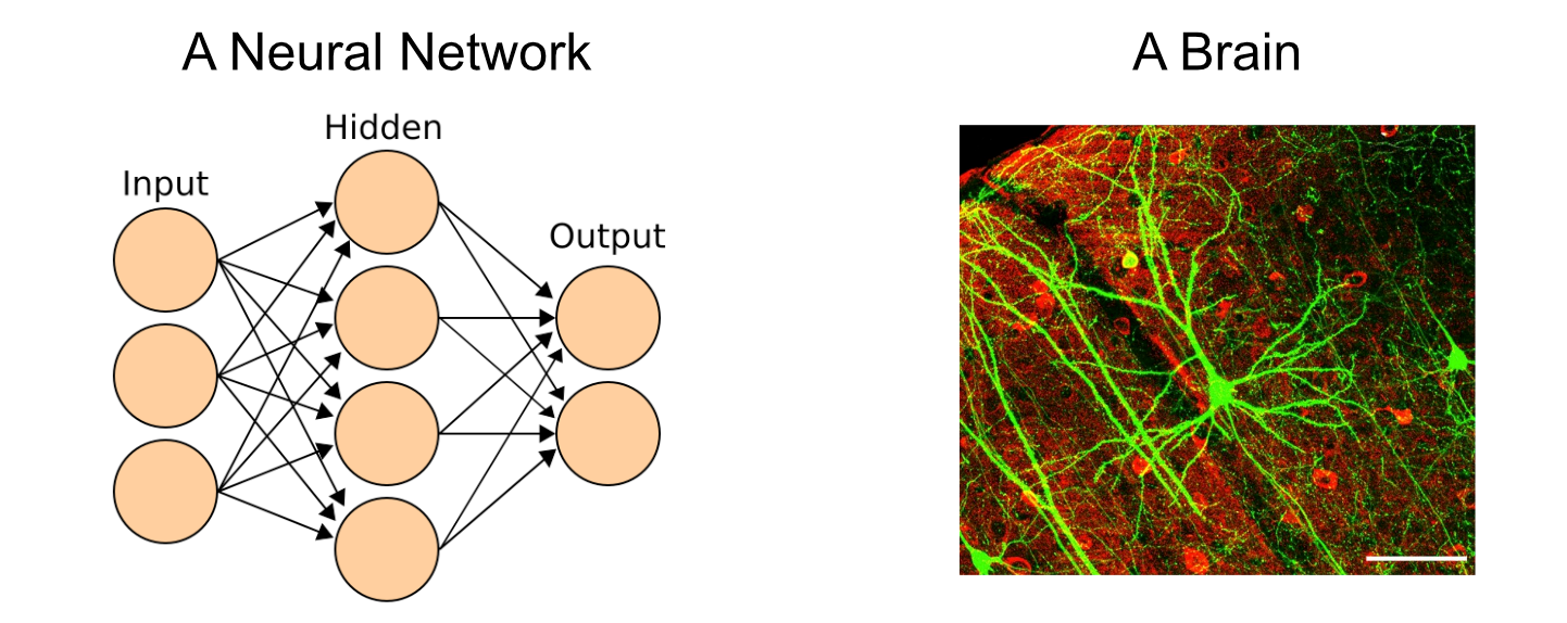
Neural networks take direct inspiration from the human brain, which is made up of billions of incredibly complex cells called neurons.

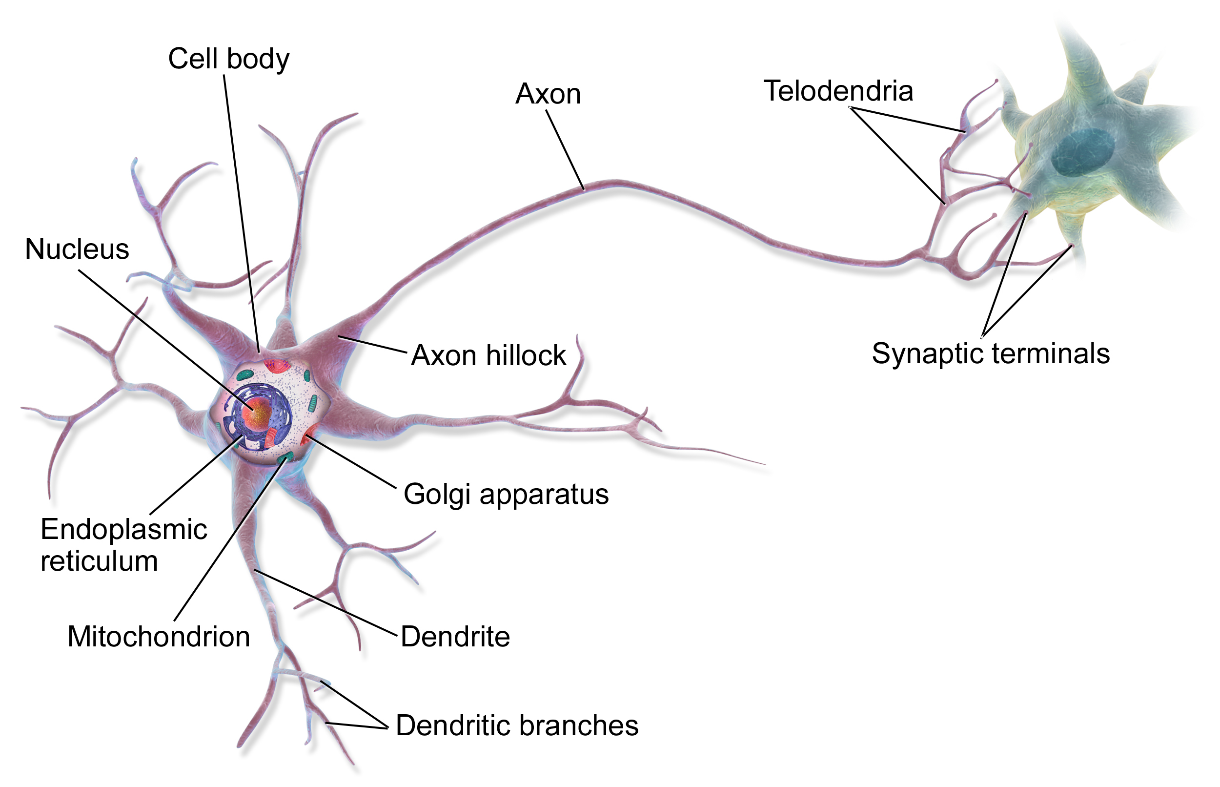
The process of thinking within the human brain is the result of communication between neurons. You might receive stimulus in the form of something you saw, then that information is propagated to neurons in the brain via electrochemical signals.

The first neurons in the brain receive that stimulus, then each neuron may choose whether or not to "fire" based on how much stimulus it received. "Firing", in this case, is a neurons decision to send signals to the neurons it’s connected to.

Then the neurons which those Neurons are connected to may or may not choose to fire.

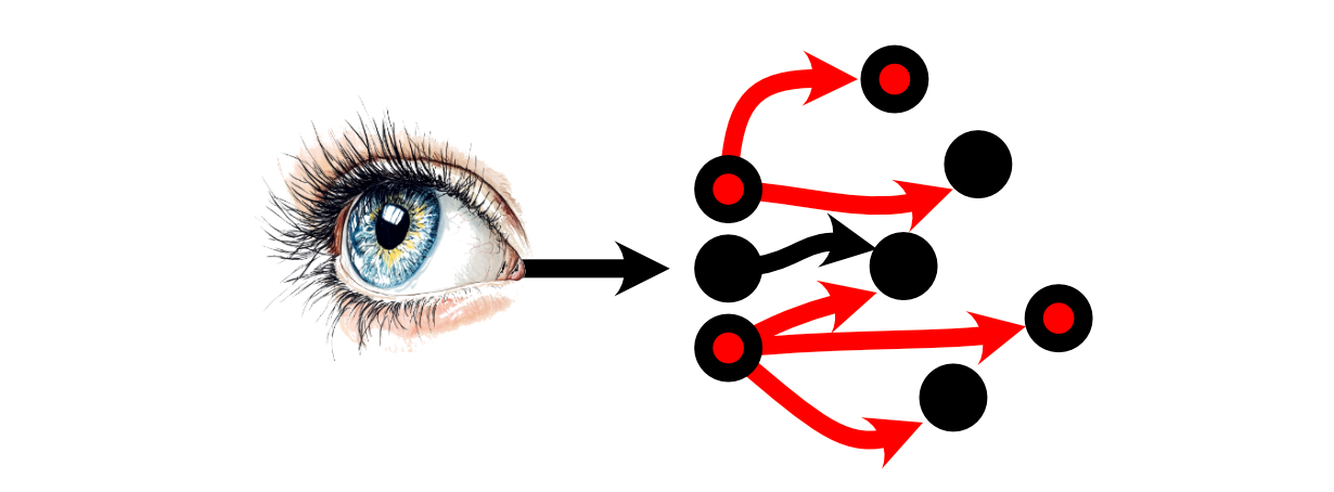
Thus, a "thought" can be conceptualized as a large number of neurons choosing to, or not to fire based on the stimulus from other neurons.

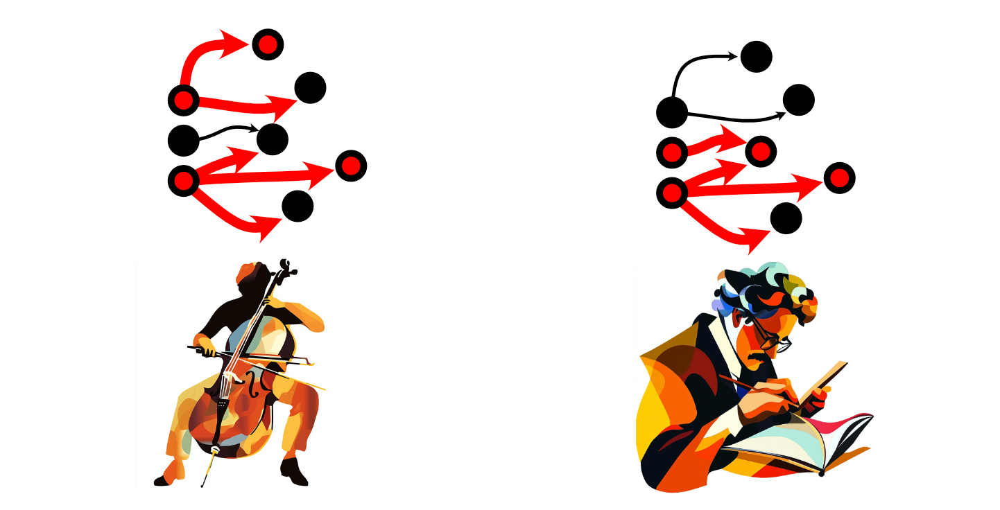
As one navigates throughout the world, one might have certain thoughts more than another person. A cellist might use some neurons more than a mathematician, for instance.

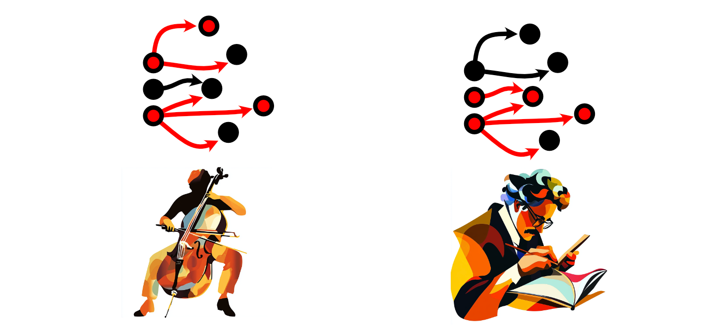
When we use certain neurons more frequently, their connections become stronger, increasing the intensity of those connections. When we don’t use certain neurons, those connections weaken. This general rule has inspired the phrase "Neurons that fire together, wire together", and is the high-level quality of the brain which is responsible for the learning process.

I’m not a neurologist, so of course this is a tremendously simplified description of the brain. However, it’s enough to understand the fundamental idea of a neural network.

The Intuition of Neural Networks

Neural networks are, essentially, a mathematically convenient and simplified version of neurons within the brain. A neural network is made up of elements called "perceptrons", which are directly inspired by neurons.

Perceptrons take in data, like a neuron does,

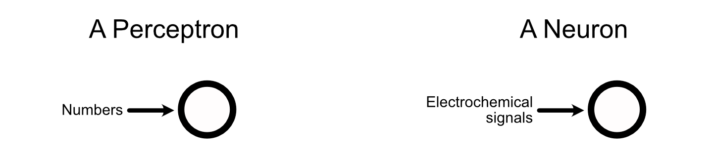
aggregate that data, like a neuron does,

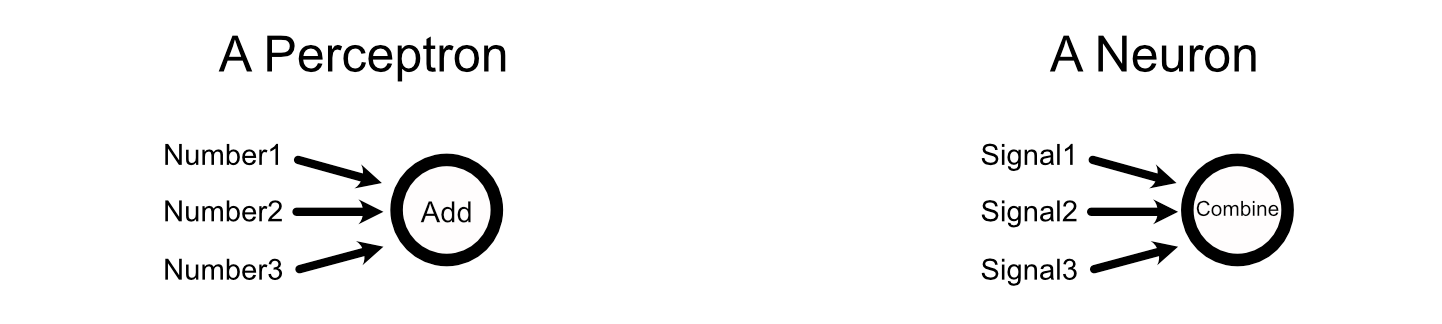
then output a signal based on the input, like a neuron does.

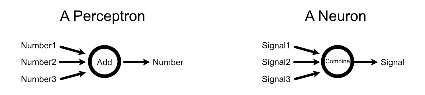
A neural network can be conceptualized as a big network of these perceptrons, just like the brain is a big network of neurons.

When a neuron in the brain fires, it does so as a binary decision. Or, in other words, neurons either fire or they don’t. Perceptrons, on the other hand, don’t "fire" per-se, but output a range of numbers based on the perceptrons input.

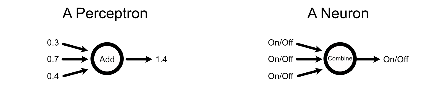
Neurons within the brain can get away with their relatively simple binary inputs and outputs because thoughts exist over time. Neurons essentially pulse at different rates, with slower and faster pulses communicating different information.

So, neurons have simple inputs and outputs in the form of on or off pulses, but the rate at which they pulse can communicate complex information. Perceptrons only see an input once per pass through the network, but their input and output can be a continuous range of values. If you’re familiar with electronics, you might reflect on how this is similar to the relationship between digital and analogue signals.

The way the math for a perceptron actually shakes out is pretty simple. A standard neural network consists of a bunch of weights connecting the perceptron’s of different layers together.

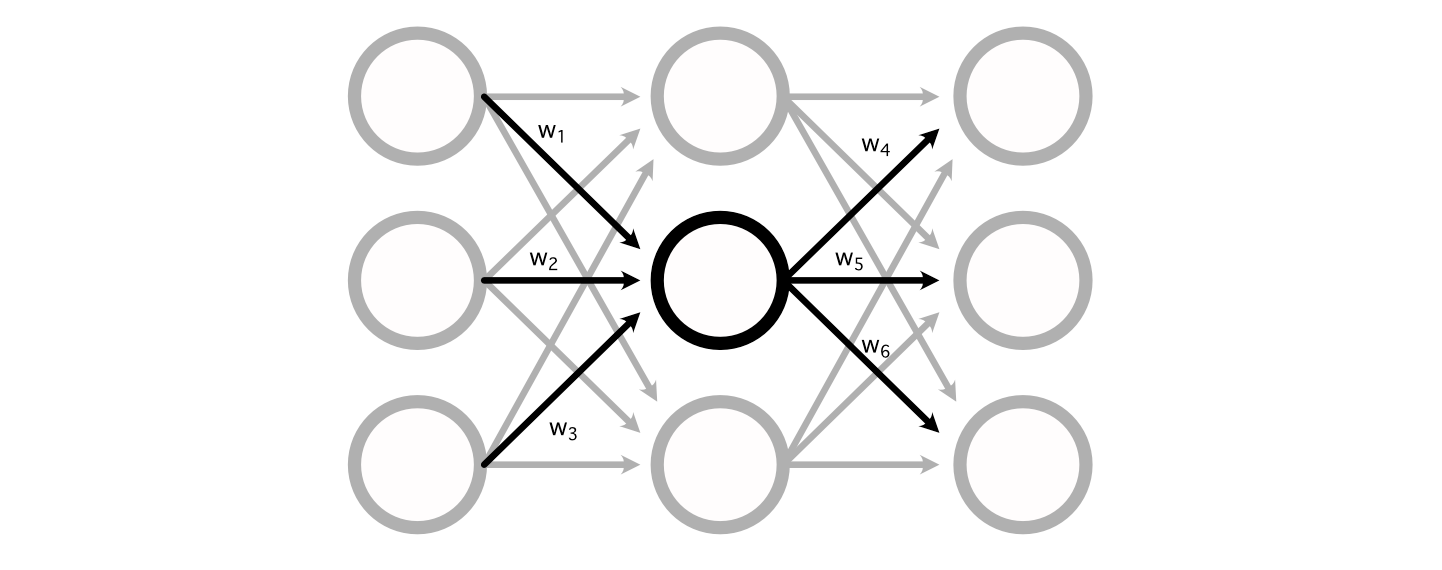
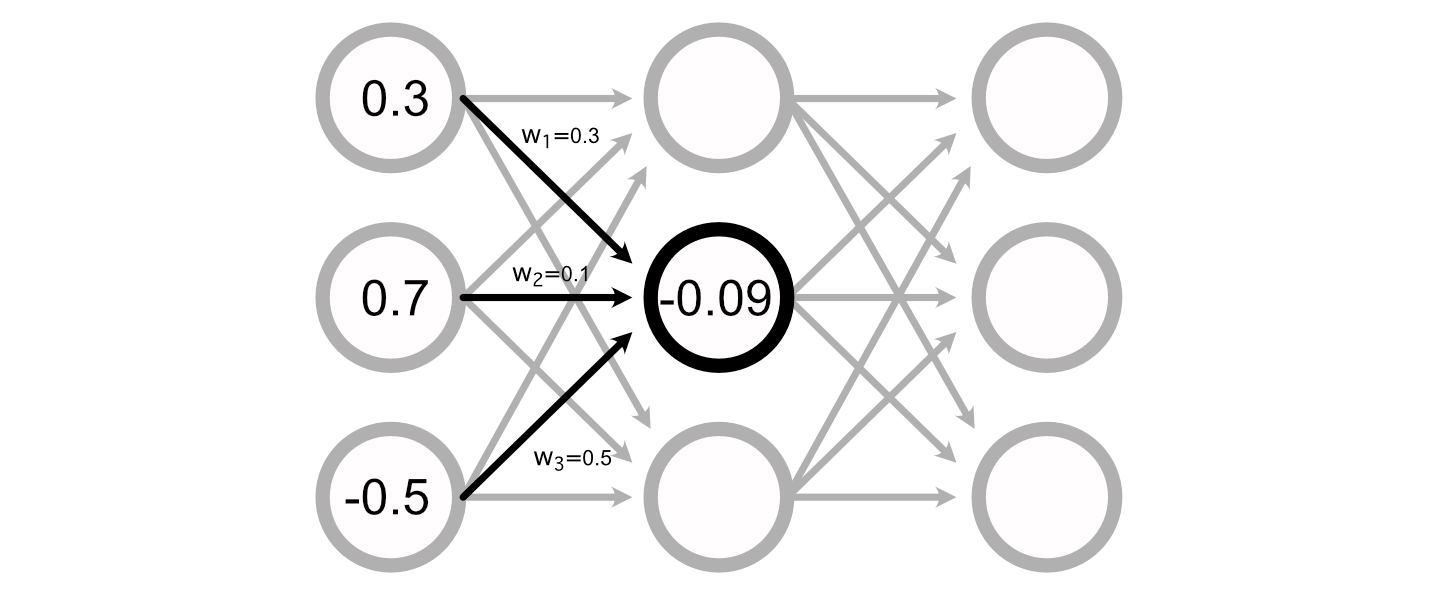
You can calculate the value of a particular perceptron by adding up all the inputs, multiplied by their respective weights.

Many Neural Networks also have a "bias" associated with each perceptron, which is added to the sum of the inputs to calculate the perceptron’s value.

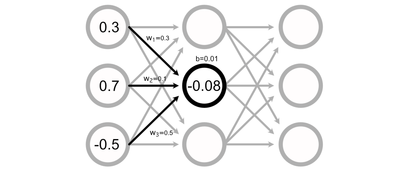
Calculating the output of a neural network, then, is just doing a bunch of addition and multiplication to calculate the value of all the perceptrons.

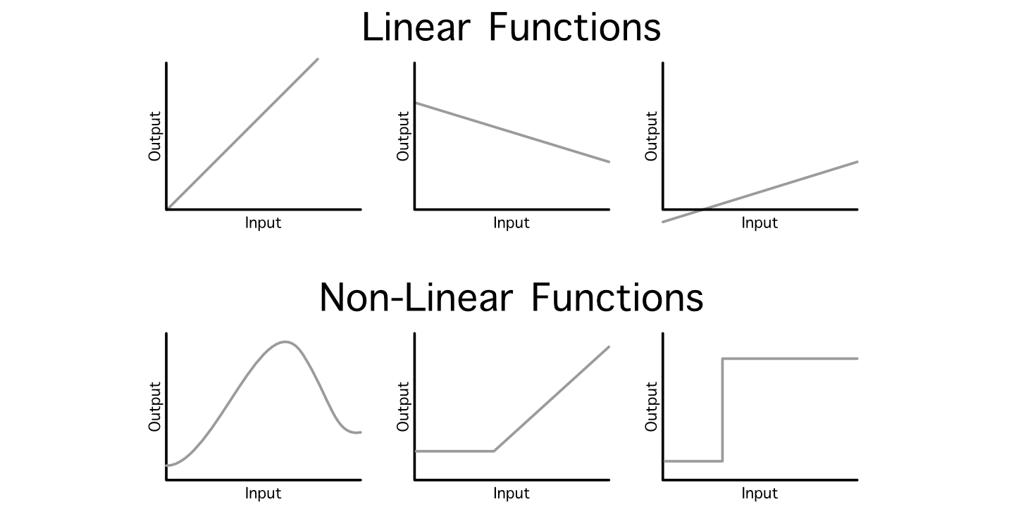
Sometimes data scientists refer to this general operation as a "linear projection", because we’re mapping an input into an output via linear operations (addition and multiplication). One problem with this approach is, even if you daisy chain a billion of these layers together, the resulting model will still just be a linear relationship between the input and output because it’s all just addition and multiplication.

This is a serious problem because not all relationships between an input and output are linear. To get around this, data scientists employ something called an "activation function". These are non-linear functions which can be injected throughout the model to, essentially, sprinkle in some non-linearity.

by interweaving non-linear activation functions between linear projections, neural networks are capable of learning very complex functions,

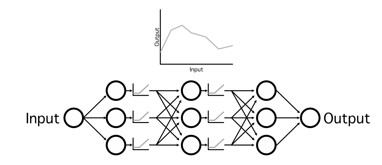
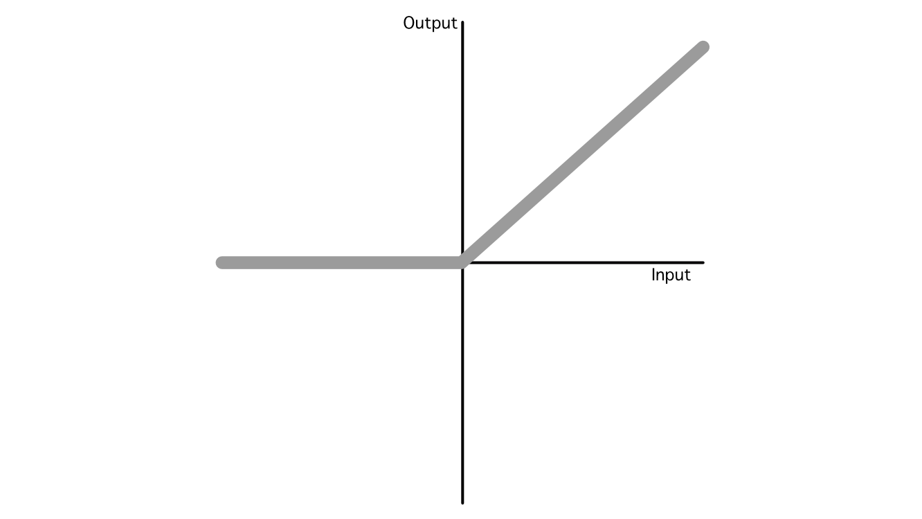
In AI there are many popular activation functions, but the industry has largely converged on three popular ones: ReLU, Sigmoid, and Softmax, which are used in a variety of different applications. Out of all of them, ReLU is the most common due to its simplicity and ability to generalize to mimic almost any other function.

So, that’s the essence of how AI models make predictions. It’s a bunch of addition and multiplication with some nonlinear functions sprinkled in between.

Another defining characteristic of neural networks is that they can be trained to be better at solving a certain problem, which we’ll explore in the next section.

Back Propagation

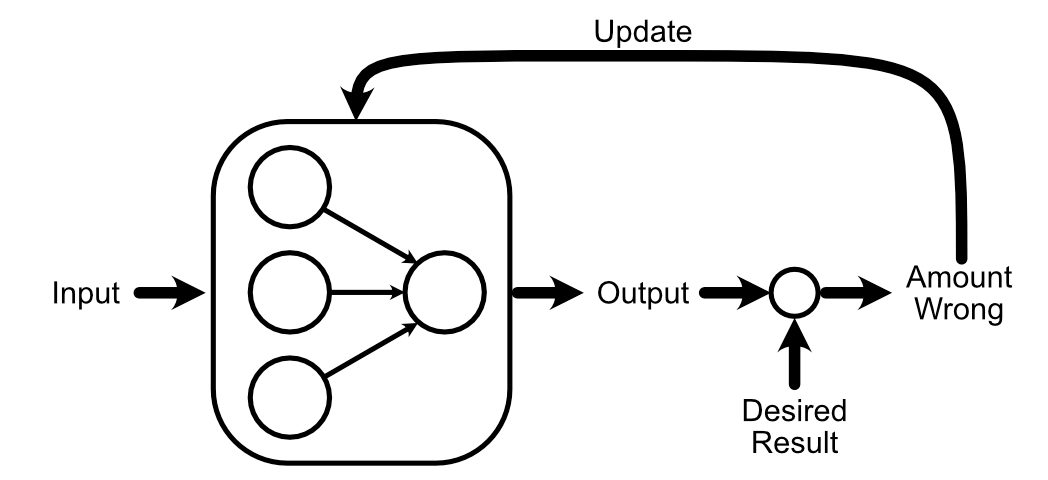
One of the fundamental ideas of AI is that you can "train" a model. This is done by asking a neural network (which starts its life as a big pile of random data) to do some task. Then, you somehow update the model based on how the model’s output compares to a known good answer.

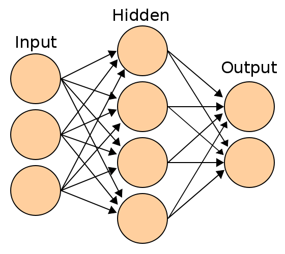
For this section, let’s imagine a neural network with an input layer, a hidden layer, and an output layer.

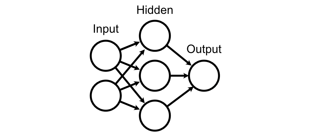
Each of these layers are connected together with, initially, completely random weights.

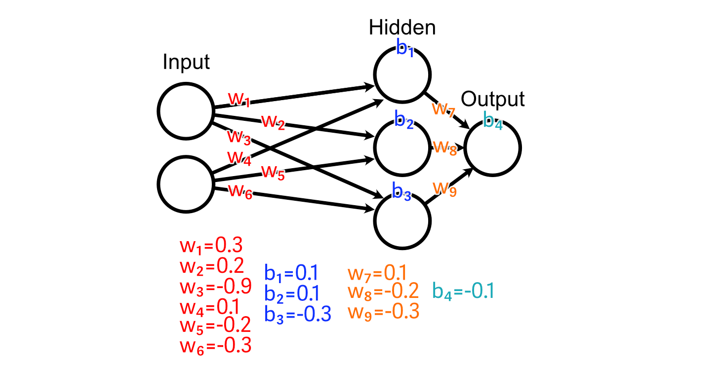
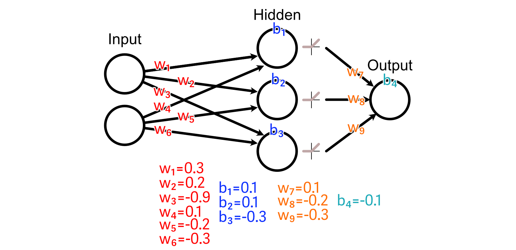
And we’ll use a ReLU activation function on our hidden layer.

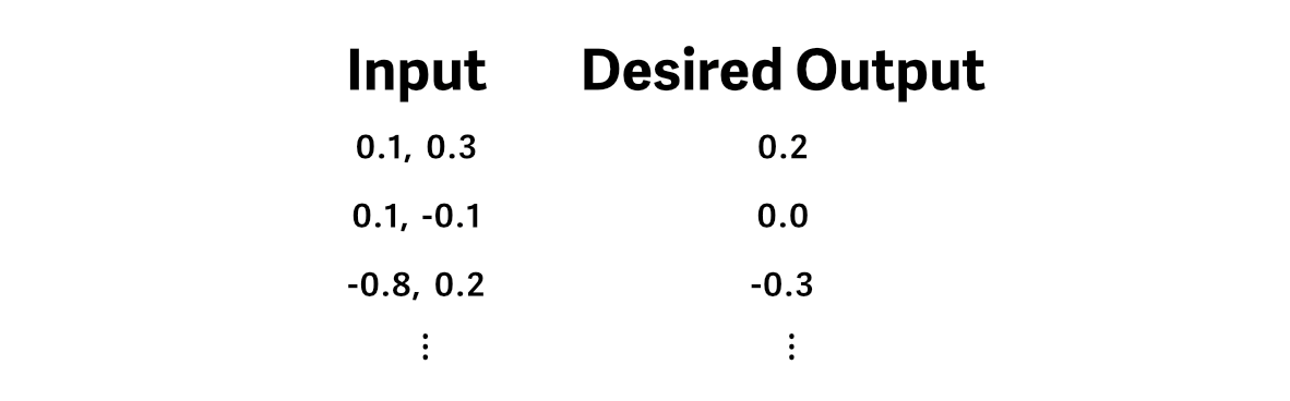
Let’s say we have some training data, in which the desired output is the average value of the input.

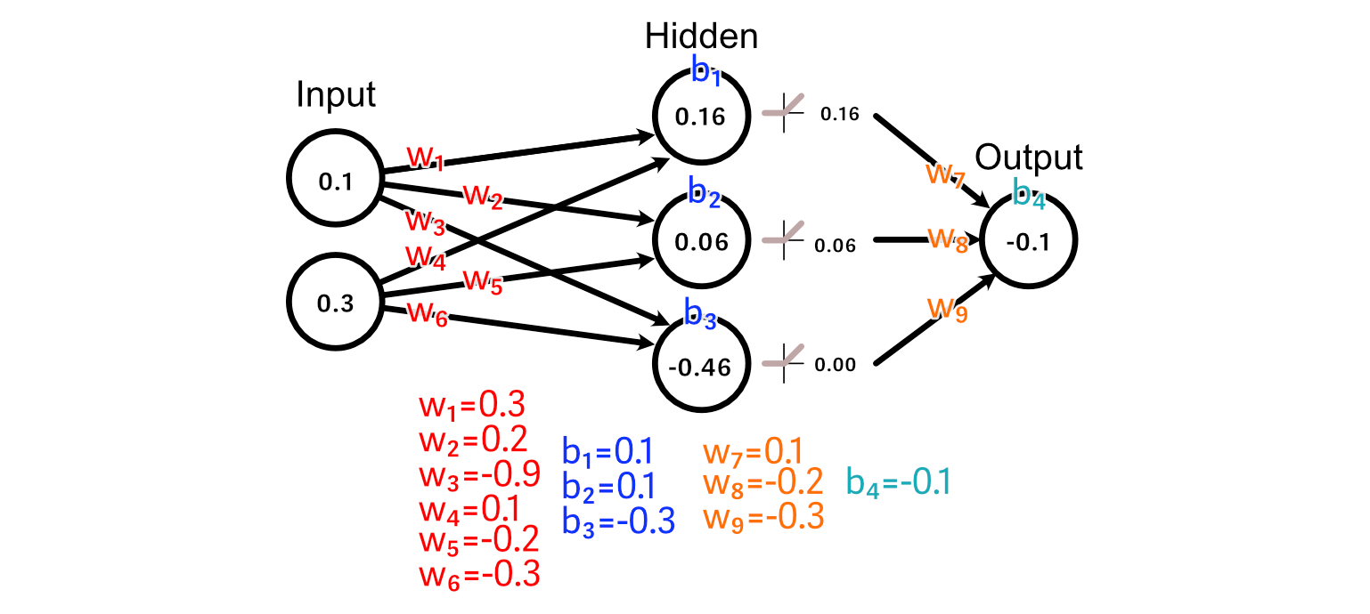
And we pass an example of our training data through the model, generating a prediction.

To make our neural network better at the task of calculating the average of the input, we first compare the predicted output to what our desired output is.

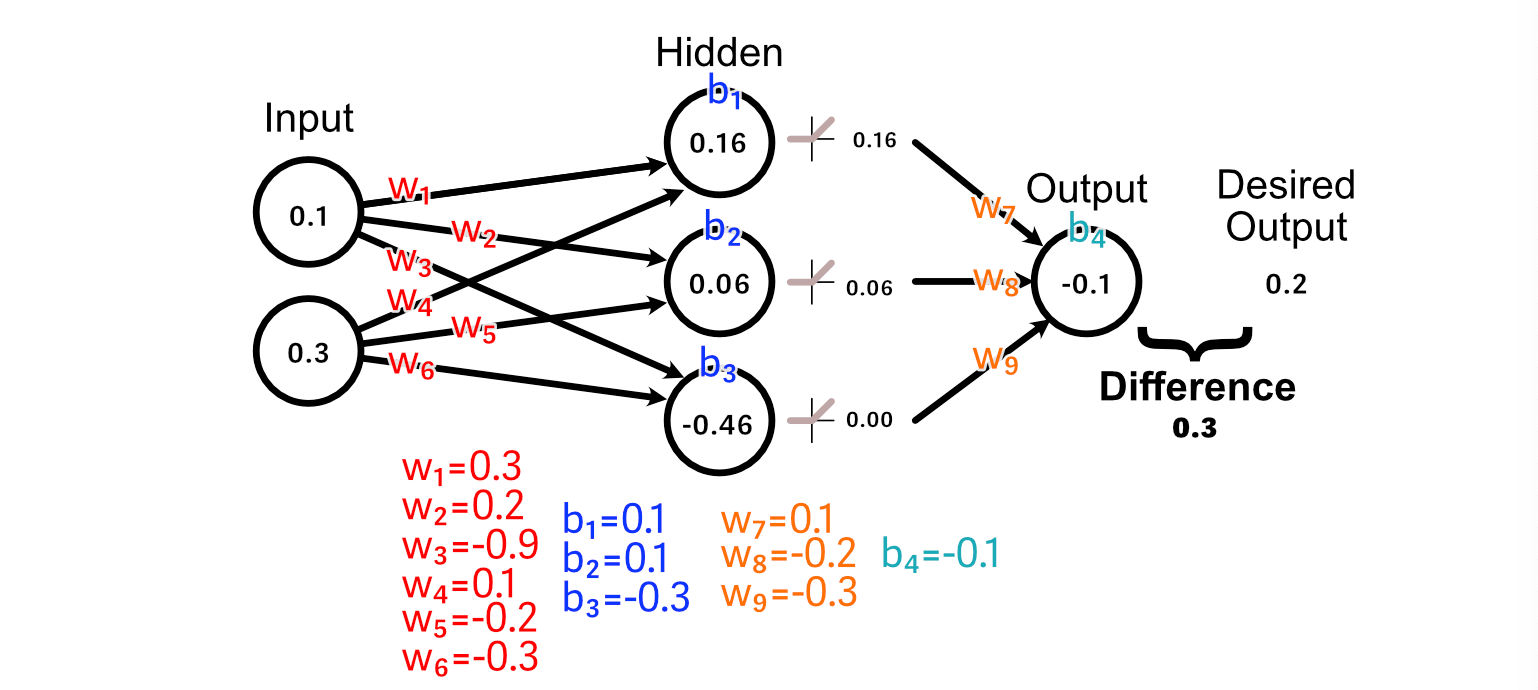
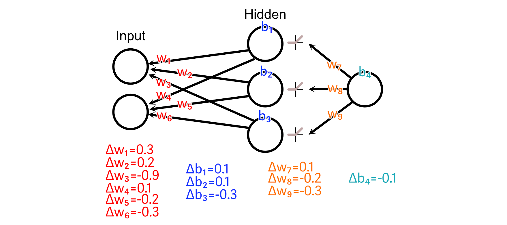
Now that we know that the output should increase in size, we can look back through the model to calculate how our weights and biases might change to promote that change.

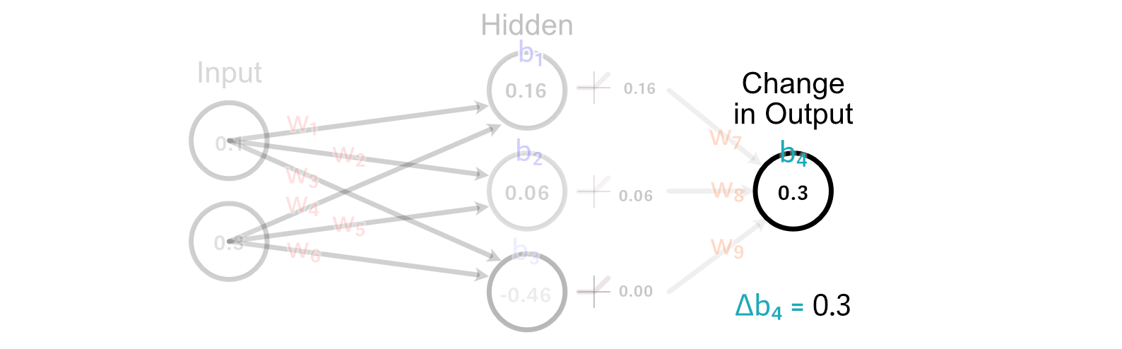
First, let’s look at the weights leading immediately into the output: w₇, w₈, w₉. Because the output of the third hidden perceptron was -0.46, the activation from ReLU was 0.00.

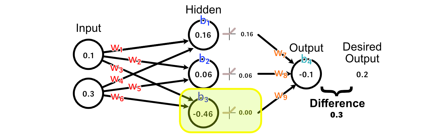
As a result, there’s no change to w₉ that could result us getting closer to our desired output, because every value of w₉ would result in a change of zero in this particular example.

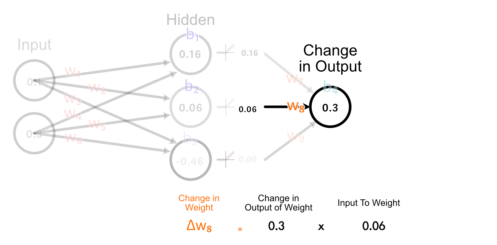
The second hidden neuron, however, does have an activated output which is greater than zero, and thus adjusting w₈ will have an impact on the output for this example.

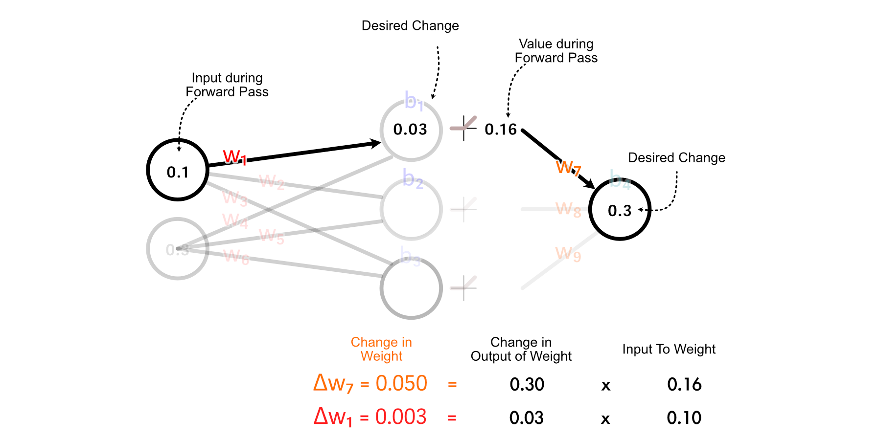
The way we actually calculate how much w₈ should change is by multiplying how much the output should change, times the input to w₈.

The easiest explanation of why we do it this way is "because calculus", but if we look at how all weights get updated in the last layer, we can form a fun intuition.

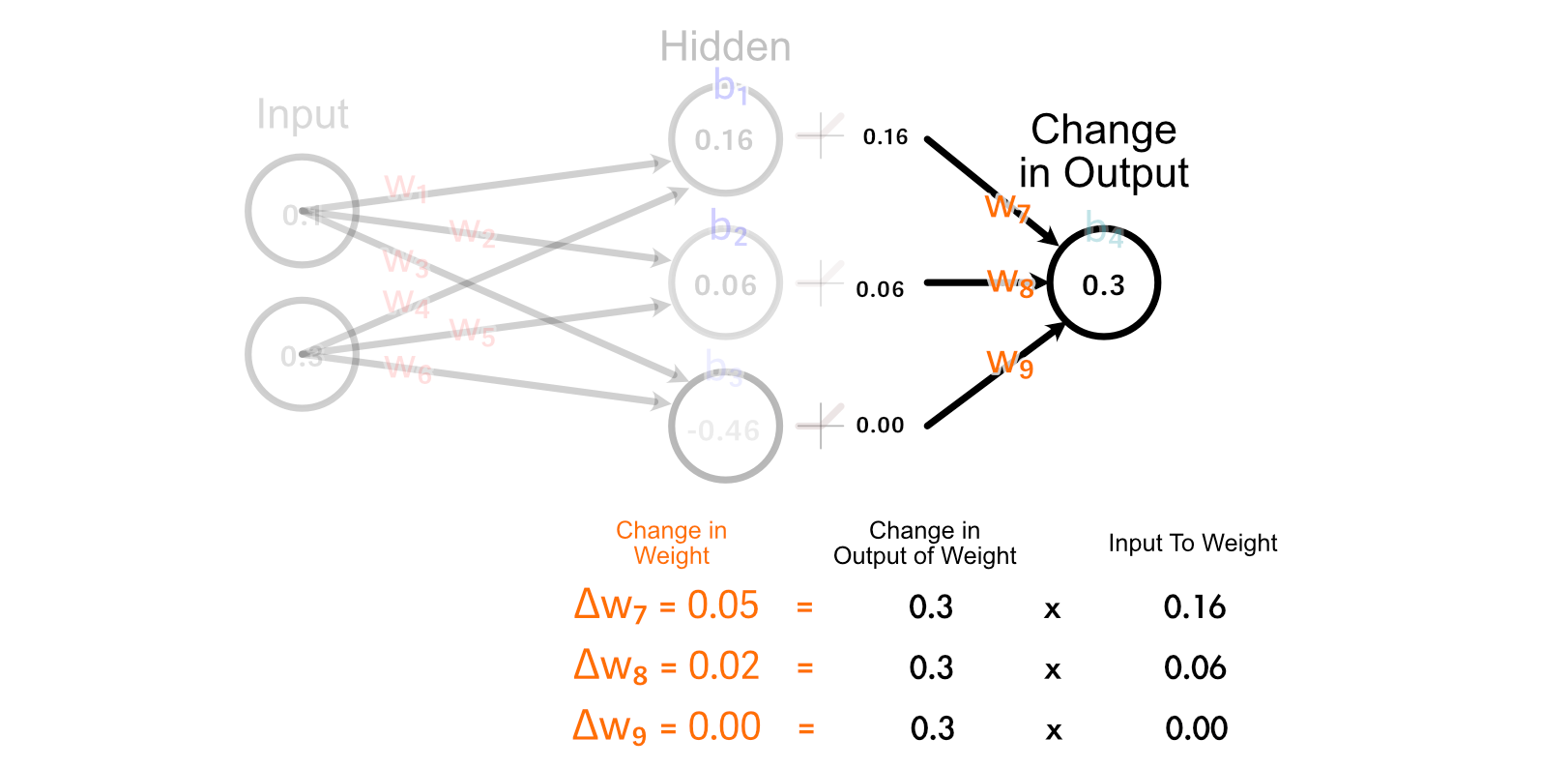
Notice how the two perceptrons that "fire" (have an output greater than zero) are updated together. Also, notice how the stronger a perceptrons output is, the more its corresponding weight is updated. This is somewhat similar to the idea that "Neurons that fire together, wire together" within the human brain.

Calculating the change to the output bias is super easy. In fact, we’ve already done it. Because the bias is how much a perceptrons output should change, the change in the bias is just the changed in the desired output. So, Δb₄=0.3

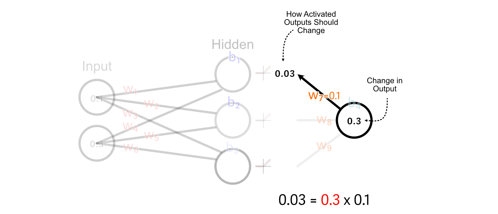
Now that we’ve calculated how the weights and bias of the output perceptron should change, we can "back propagate" our desired change in output through the model. Let’s start with back propagating so we can calculate how we should update w₁.

First, we calculate how the activated output of the of the first hidden neuron should change. We do that by multiplying the change in output by w₇.

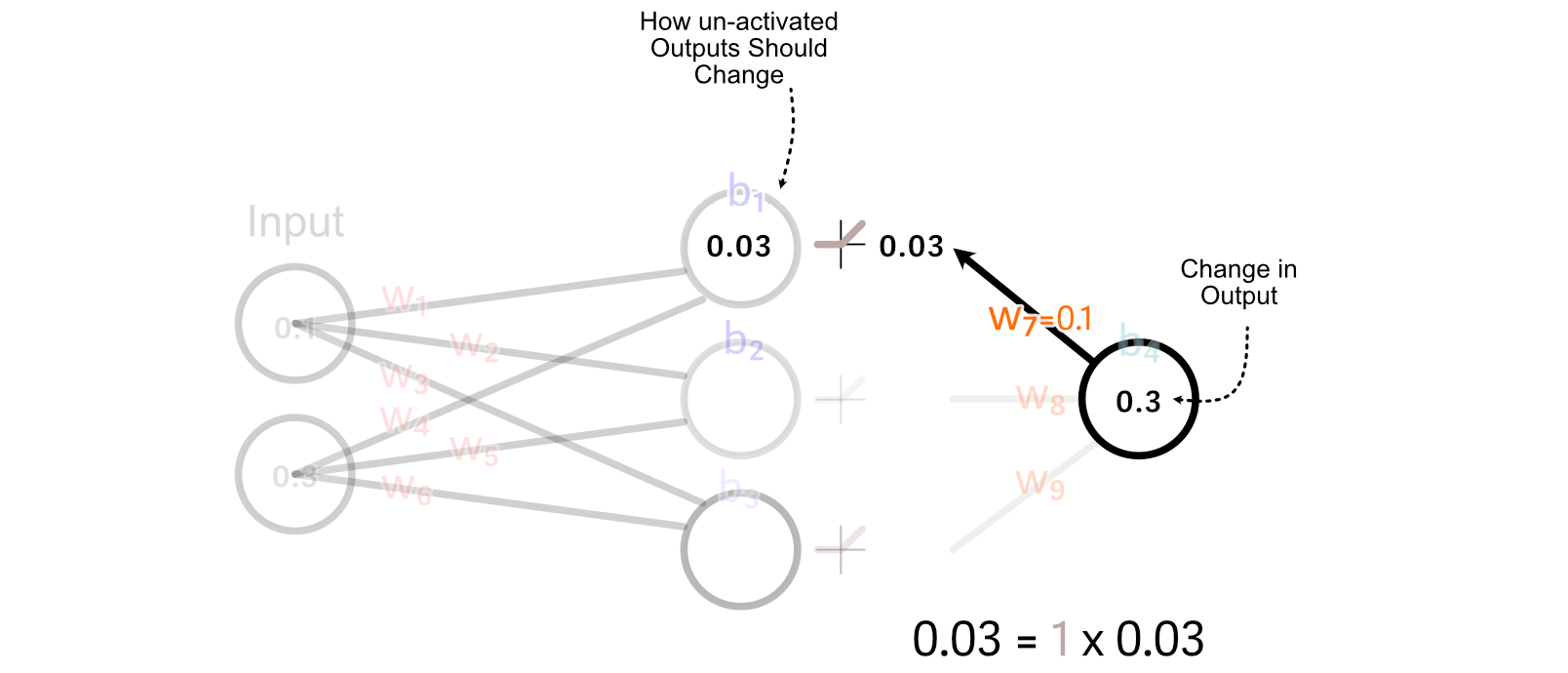
For values that are greater than zero, ReLU simply multiplies those values by 1. So, for this example, the change we want the un-activated value of the first hidden neuron is equal to the desired change in the activated output

Recall that we calculated how to update w₇ based on multiplying it’s input by the change in its desired output. We can do the same thing to calculate the change in w₁.

It’s important to note, we’re not actually updating any of the weights or biases throughout this process. Rather, we’re taking a tally of how we should update each parameter, assuming no other parameters are updated.

So, we can do those calculations to calculate all parameter changes.

A fundamental idea of back propagation is called "Learning Rate", which concerns the size of the changes we make to neural networks based on a particular batch of data. To explain why this is important, I’d like to use an analogy.

Imagine you went outside one day, and everyone wearing a hat gave you a funny look. You probably don’t want to jump to the conclusion that wearing hat = funny look , but you might be a bit skeptical of people wearing hats. After three, four, five days, a month, or even a year, if it seems like the vast majority of people wearing hats are giving you a funny look, you may start considering that a strong trend.

Similarly, when we train a neural network, we don’t want to completely change how the neural network thinks based on a single training example. Rather, we want each batch to only incrementally change how the model thinks. As we expose the model to many examples, we would hope that the model would learn important trends within the data.

After we’ve calculated how each parameter should change as if it were the only parameter being updated, we can multiply all those changes by a small number, like 0.001 , before applying those changes to the parameters. This small number is commonly referred to as the "learning rate", and the exact value it should have is dependent on the model we’re training on. This effectively scales down our adjustments before applying them to the model.

At this point we covered pretty much everything one would need to know to implement a neural network. Let’s give it a shot!

Implementing a Neural Network from Scratch

Typically, a data scientist would just use a library like PyTorch to implement a neural network in a few lines of code, but we’ll be defining a neural network from the ground up using NumPy, a numerical computing library.

First, let’s start with a way to define the structure of the neural network.

"""Blocking out the structure of the Neural Network
"""

import numpy as np

class SimpleNN:
    def __init__(self, architecture):
        self.architecture = architecture
        self.weights = []
        self.biases = []

        # Initialize weights and biases
        np.random.seed(99)
        for i in range(len(architecture) - 1):
            self.weights.append(np.random.uniform(
                low=-1, high=1,
                size=(architecture[i], architecture[i+1])
            ))
            self.biases.append(np.zeros((1, architecture[i+1])))

architecture = [2, 64, 64, 64, 1]  # Two inputs, two hidden layers, one output
model = SimpleNN(architecture)

print('weight dimensions:')
for w in model.weights:
    print(w.shape)

print('nbias dimensions:')
for b in model.biases:
    print(b.shape)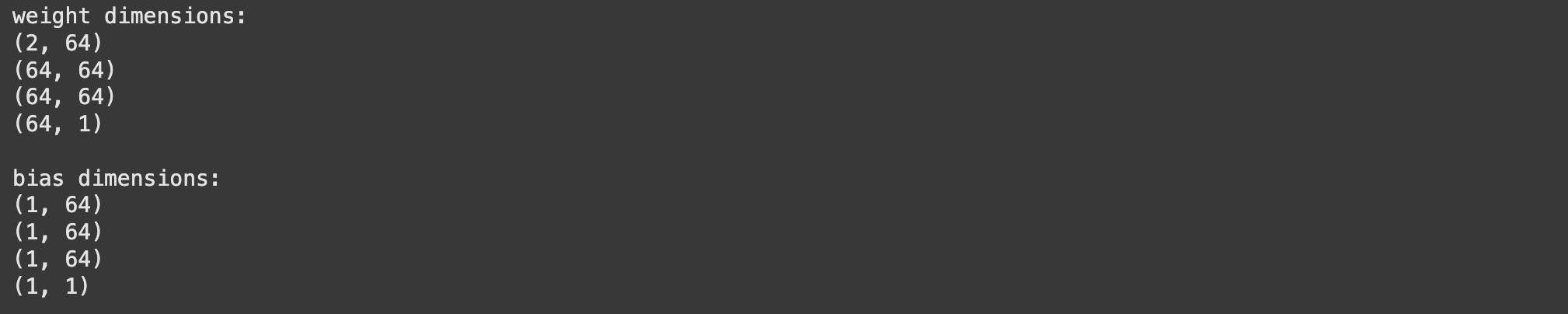

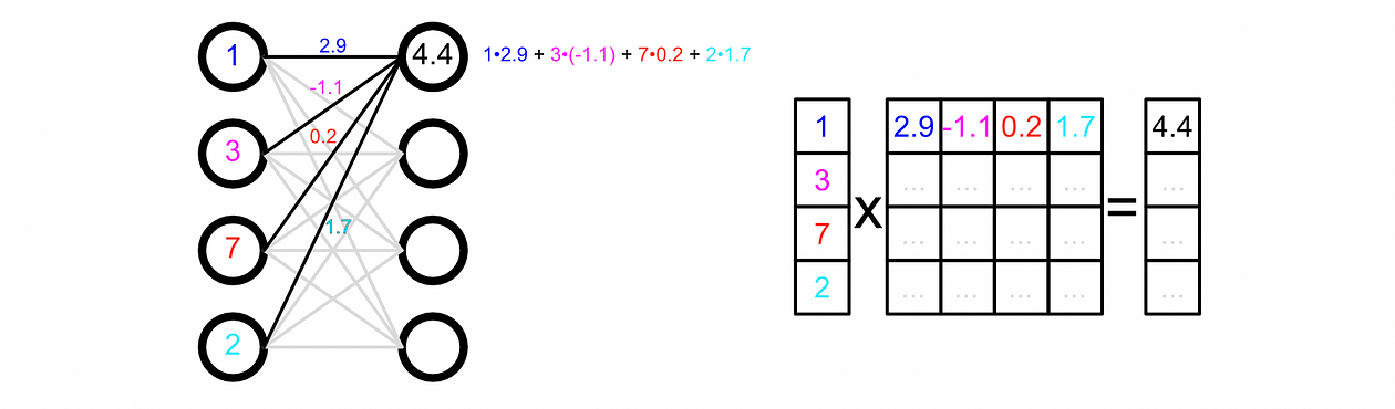
While we typically draw neural networks as a dense web in reality we represent the weights between their connections as matrices. This is convenient because matrix multiplication, then, is equivalent to passing data through a neural network.

We can make our model make a prediction based on some input by passing the input through each layer.

"""Implementing the Forward Pass
"""

import numpy as np

class SimpleNN:
    def __init__(self, architecture):
        self.architecture = architecture
        self.weights = []
        self.biases = []

        # Initialize weights and biases
        np.random.seed(99)
        for i in range(len(architecture) - 1):
            self.weights.append(np.random.uniform(
                low=-1, high=1,
                size=(architecture[i], architecture[i+1])
            ))
            self.biases.append(np.zeros((1, architecture[i+1])))

    @staticmethod
    def relu(x):
        #implementing the relu activation function
        return np.maximum(0, x)

    def forward(self, X):
        #iterating through all layers
        for W, b in zip(self.weights, self.biases):

            #applying the weight and bias of the layer
            X = np.dot(X, W) + b

            #doing ReLU for all but the last layer
            if W is not self.weights[-1]:
                X = self.relu(X)

        #returning the result
        return X

    def predict(self, X):
        y = self.forward(X)
        return y.flatten()

#defining a model
architecture = [2, 64, 64, 64, 1]  # Two inputs, two hidden layers, one output
model = SimpleNN(architecture)

# Generate predictions
prediction = model.predict(np.array([0.1,0.2]))
print(prediction)

We need to be able to train this model, and to do that we’ll first need a problem to train the model on. I defined a random function that takes in two inputs and results in an output:

"""Defining what we want the model to learn
"""
import numpy as np
import matplotlib.pyplot as plt

# Define a random function with two inputs
def random_function(x, y):
    return (np.sin(x) + x * np.cos(y) + y + 3**(x/3))

# Generate a grid of x and y values
x = np.linspace(-10, 10, 100)
y = np.linspace(-10, 10, 100)
X, Y = np.meshgrid(x, y)

# Compute the output of the random function
Z = random_function(X, Y)

# Create a 2D plot
plt.figure(figsize=(8, 6))
contour = plt.contourf(X, Y, Z, cmap='viridis')
plt.colorbar(contour, label='Function Value')
plt.title('2D Plot of Objective Function')
plt.xlabel('X-axis')
plt.ylabel('Y-axis')
plt.show()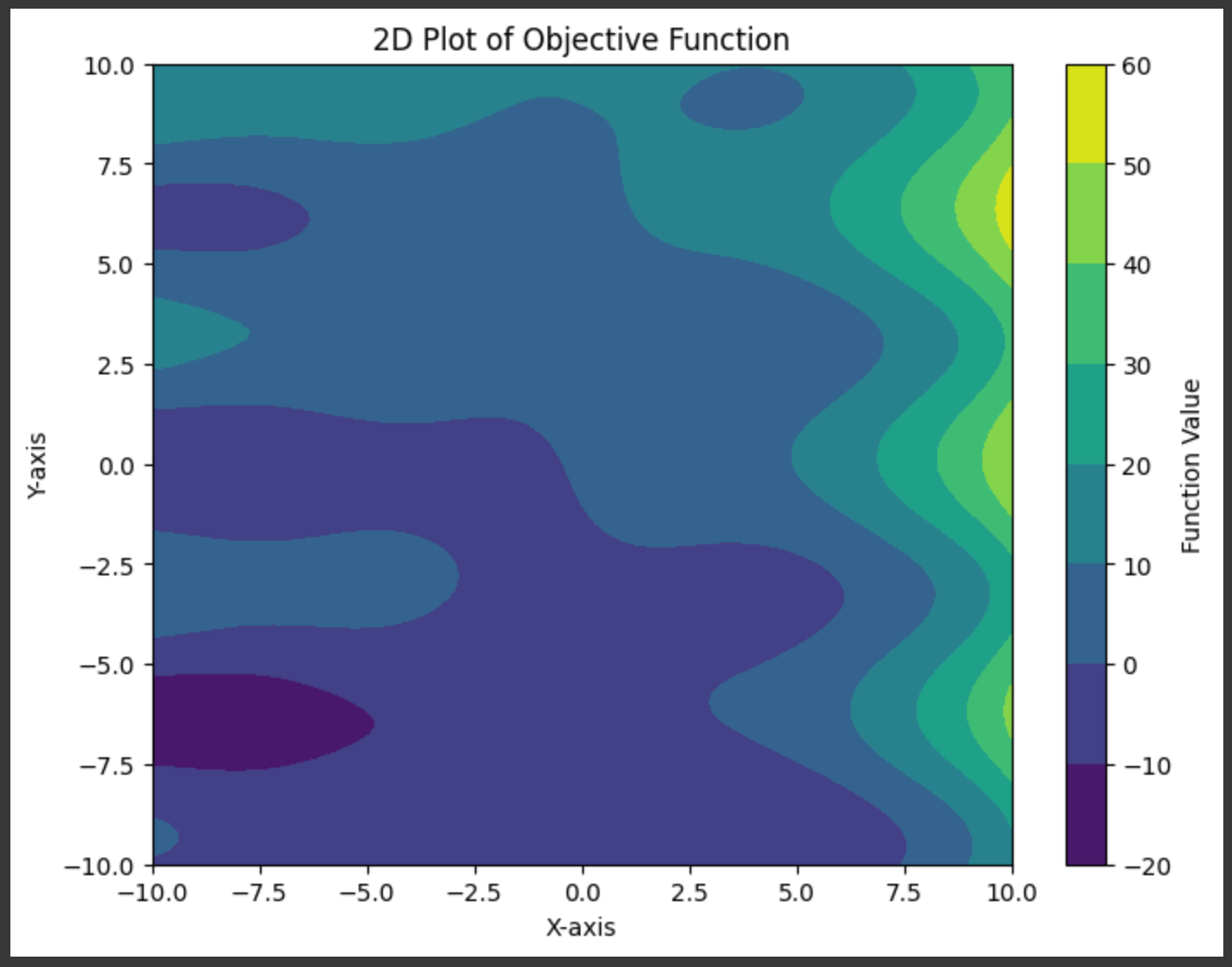

In the real world we wouldn’t know the underlying function. We can mimic that reality by creating a dataset consisting of random points:

import numpy as np
import pandas as pd
import matplotlib.pyplot as plt

# Define a random function with two inputs
def random_function(x, y):
    return (np.sin(x) + x * np.cos(y) + y + 3**(x/3))

# Define the number of random samples to generate
n_samples = 1000

# Generate random X and Y values within a specified range
x_min, x_max = -10, 10
y_min, y_max = -10, 10

# Generate random values for X and Y
X_random = np.random.uniform(x_min, x_max, n_samples)
Y_random = np.random.uniform(y_min, y_max, n_samples)

# Evaluate the random function at the generated X and Y values
Z_random = random_function(X_random, Y_random)

# Create a dataset
dataset = pd.DataFrame({
    'X': X_random,
    'Y': Y_random,
    'Z': Z_random
})

# Display the dataset
print(dataset.head())

# Create a 2D scatter plot of the sampled data
plt.figure(figsize=(8, 6))
scatter = plt.scatter(dataset['X'], dataset['Y'], c=dataset['Z'], cmap='viridis', s=10)
plt.colorbar(scatter, label='Function Value')
plt.title('Scatter Plot of Randomly Sampled Data')
plt.xlabel('X-axis')
plt.ylabel('Y-axis')
plt.show()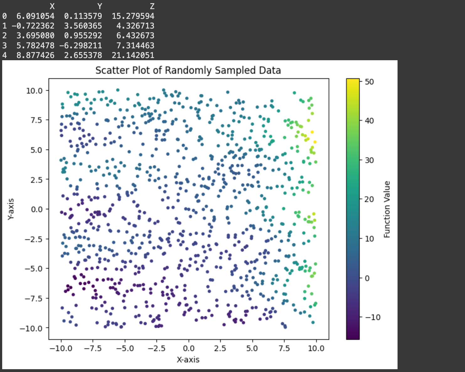

Recall that the back propagation algorithm updates parameters based on what happens in a forward pass. So, before we implement backpropagation itself, let’s keep track of a few important values in the forward pass: The inputs and outputs of each perceptron throughout the model.

import numpy as np

class SimpleNN:
    def __init__(self, architecture):
        self.architecture = architecture
        self.weights = []
        self.biases = []

        #keeping track of these values in this code block
        #so we can observe them
        self.perceptron_inputs = None
        self.perceptron_outputs = None

        # Initialize weights and biases
        np.random.seed(99)
        for i in range(len(architecture) - 1):
            self.weights.append(np.random.uniform(
                low=-1, high=1,
                size=(architecture[i], architecture[i+1])
            ))
            self.biases.append(np.zeros((1, architecture[i+1])))

    @staticmethod
    def relu(x):
        return np.maximum(0, x)

    def forward(self, X):
        self.perceptron_inputs = [X]
        self.perceptron_outputs = []

        for W, b in zip(self.weights, self.biases):
            Z = np.dot(self.perceptron_inputs[-1], W) + b
            self.perceptron_outputs.append(Z)

            if W is self.weights[-1]:  # Last layer (output)
                A = Z  # Linear output for regression
            else:
                A = self.relu(Z)
            self.perceptron_inputs.append(A)

        return self.perceptron_inputs, self.perceptron_outputs

    def predict(self, X):
        perceptron_inputs, _ = self.forward(X)
        return perceptron_inputs[-1].flatten()

#defining a model
architecture = [2, 64, 64, 64, 1]  # Two inputs, two hidden layers, one output
model = SimpleNN(architecture)

# Generate predictions
prediction = model.predict(np.array([0.1,0.2]))

#looking through critical optimization values
for i, (inpt, outpt) in enumerate(zip(model.perceptron_inputs, model.perceptron_outputs[:-1])):
    print(f'layer {i}')
    print(f'input: {inpt.shape}')
    print(f'output: {outpt.shape}')
    print('')

print('Final Output:')
print(model.perceptron_outputs[-1].shape)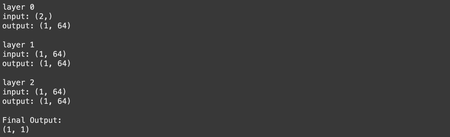

Now that we have a record stored of critical intermediary value within the network, we can use those values, along with the error of a model for a particular prediction, to calculate the changes we should make to the model.

import numpy as np

class SimpleNN:
    def __init__(self, architecture):
        self.architecture = architecture
        self.weights = []
        self.biases = []

        # Initialize weights and biases
        np.random.seed(99)
        for i in range(len(architecture) - 1):
            self.weights.append(np.random.uniform(
                low=-1, high=1,
                size=(architecture[i], architecture[i+1])
            ))
            self.biases.append(np.zeros((1, architecture[i+1])))

    @staticmethod
    def relu(x):
        return np.maximum(0, x)

    @staticmethod
    def relu_as_weights(x):
        return (x > 0).astype(float)

    def forward(self, X):
        perceptron_inputs = [X]
        perceptron_outputs = []

        for W, b in zip(self.weights, self.biases):
            Z = np.dot(perceptron_inputs[-1], W) + b
            perceptron_outputs.append(Z)

            if W is self.weights[-1]:  # Last layer (output)
                A = Z  # Linear output for regression
            else:
                A = self.relu(Z)
            perceptron_inputs.append(A)

        return perceptron_inputs, perceptron_outputs

    def backward(self, perceptron_inputs, perceptron_outputs, target):
        weight_changes = []
        bias_changes = []

        m = len(target)
        dA = perceptron_inputs[-1] - target.reshape(-1, 1)  # Output layer gradient

        for i in reversed(range(len(self.weights))):
            dZ = dA if i == len(self.weights) - 1 else dA * self.relu_as_weights(perceptron_outputs[i])
            dW = np.dot(perceptron_inputs[i].T, dZ) / m
            db = np.sum(dZ, axis=0, keepdims=True) / m
            weight_changes.append(dW)
            bias_changes.append(db)

            if i > 0:
                dA = np.dot(dZ, self.weights[i].T)

        return list(reversed(weight_changes)), list(reversed(bias_changes))

    def predict(self, X):
        perceptron_inputs, _ = self.forward(X)
        return perceptron_inputs[-1].flatten()

#defining a model
architecture = [2, 64, 64, 64, 1]  # Two inputs, two hidden layers, one output
model = SimpleNN(architecture)

#defining a sample input and target output
input = np.array([[0.1,0.2]])
desired_output = np.array([0.5])

#doing forward and backward pass to calculate changes
perceptron_inputs, perceptron_outputs = model.forward(input)
weight_changes, bias_changes = model.backward(perceptron_inputs, perceptron_outputs, desired_output)

#smaller numbers for printing
np.set_printoptions(precision=2)

for i, (layer_weights, layer_biases, layer_weight_changes, layer_bias_changes)
in enumerate(zip(model.weights, model.biases, weight_changes, bias_changes)):
    print(f'layer {i}')
    print(f'weight matrix: {layer_weights.shape}')
    print(f'weight matrix changes: {layer_weight_changes.shape}')
    print(f'bias matrix: {layer_biases.shape}')
    print(f'bias matrix changes: {layer_bias_changes.shape}')
    print('')

print('The weight and weight change matrix of the second layer:')
print('weight matrix:')
print(model.weights[1])
print('change matrix:')
print(weight_changes[1])

This is probably the most complex implementation step, so I want to take a moment to dig through some of the details. The fundamental idea is exactly as we described in previous sections. We’re iterating over all layers, from back to front, and calculating what change to each weight and bias would result in a better output.

# calculating output error
dA = perceptron_inputs[-1] - target.reshape(-1, 1)

#a scaling factor for the batch size.
#you want changes to be an average across all batches
#so we divide by m once we've aggregated all changes.
m = len(target)

for i in reversed(range(len(self.weights))):
  dZ = dA #simplified for now

  # calculating change to weights
  dW = np.dot(perceptron_inputs[i].T, dZ) / m
  # calculating change to bias
  db = np.sum(dZ, axis=0, keepdims=True) / m

  # keeping track of required changes
  weight_changes.append(dW)
  bias_changes.append(db)
  ...

Calculating the change to bias is pretty straight forward. If you look at how the output of a given neuron should have impacted all future neurons, you can add up all those values (which are both positive and negative) to get an idea of if the neuron should be biased in a positive or negative direction.

The way we calculate the change to weights, by using matrix multiplication, is a bit more mathematically complex.

dW = np.dot(perceptron_inputs[i].T, dZ) / m

Basically, this line says that the change in the weight should be equal to the value going into the perceptron, times how much the output should have changed. If a perceptron had a big input, the change to its outgoing weights should be a large magnitude, if the perceptron had a small input, the change to its outgoing weights will be small. Also, if a weight points towards an output which should change a lot, the weight should change a lot.

There is another line we should discuss in our back propagation implement.

dZ = dA if i == len(self.weights) - 1 else dA * self.relu_as_weights(perceptron_outputs[i])

In this particular network, there are activation functions throughout the network, following all but the final output. When we do back propagation, we need to back-propagate through these activation functions so that we can update the neurons which lie before them. We do this for all but the last layer, which doesn’t have an activation function, which is why dZ = dA if i == len(self.weights) - 1 .

In fancy math speak we would call this a derivative, but because I don’t want to get into calculus, I called the function relu_as_weights . Basically, we can treat each of our ReLU activations as something like a tiny neural network, who’s weight is a function of the input. If the input of the ReLU activation function is less than zero, then that’s like passing that input through a neural network with a weight of zero. If the input of ReLU is greater than zero, then that’s like passing the input through a neural netowork with a weight of one.

This is exactly what the relu_as_weights function does.

def relu_as_weights(x):
        return (x > 0).astype(float)

Using this logic we can treat back propagating through ReLU just like we back propagate through the rest of the neural network.

Again, I’ll be covering this concept from a more robust mathematical prospective soon, but that’s the essential idea from a conceptual perspective.

Now that we have the forward and backward pass implemented, we can implement training the model.

import numpy as np

class SimpleNN:
    def __init__(self, architecture):
        self.architecture = architecture
        self.weights = []
        self.biases = []

        # Initialize weights and biases
        np.random.seed(99)
        for i in range(len(architecture) - 1):
            self.weights.append(np.random.uniform(
                low=-1, high=1,
                size=(architecture[i], architecture[i+1])
            ))
            self.biases.append(np.zeros((1, architecture[i+1])))

    @staticmethod
    def relu(x):
        return np.maximum(0, x)

    @staticmethod
    def relu_as_weights(x):
        return (x > 0).astype(float)

    def forward(self, X):
        perceptron_inputs = [X]
        perceptron_outputs = []

        for W, b in zip(self.weights, self.biases):
            Z = np.dot(perceptron_inputs[-1], W) + b
            perceptron_outputs.append(Z)

            if W is self.weights[-1]:  # Last layer (output)
                A = Z  # Linear output for regression
            else:
                A = self.relu(Z)
            perceptron_inputs.append(A)

        return perceptron_inputs, perceptron_outputs

    def backward(self, perceptron_inputs, perceptron_outputs, y_true):
        weight_changes = []
        bias_changes = []

        m = len(y_true)
        dA = perceptron_inputs[-1] - y_true.reshape(-1, 1)  # Output layer gradient

        for i in reversed(range(len(self.weights))):
            dZ = dA if i == len(self.weights) - 1 else dA * self.relu_as_weights(perceptron_outputs[i])
            dW = np.dot(perceptron_inputs[i].T, dZ) / m
            db = np.sum(dZ, axis=0, keepdims=True) / m
            weight_changes.append(dW)
            bias_changes.append(db)

            if i > 0:
                dA = np.dot(dZ, self.weights[i].T)

        return list(reversed(weight_changes)), list(reversed(bias_changes))

    def update_weights(self, weight_changes, bias_changes, lr):
        for i in range(len(self.weights)):
            self.weights[i] -= lr * weight_changes[i]
            self.biases[i] -= lr * bias_changes[i]

    def train(self, X, y, epochs, lr=0.01):
        for epoch in range(epochs):
            perceptron_inputs, perceptron_outputs = self.forward(X)
            weight_changes, bias_changes = self.backward(perceptron_inputs, perceptron_outputs, y)
            self.update_weights(weight_changes, bias_changes, lr)

            if epoch % 20 == 0 or epoch == epochs - 1:
                loss = np.mean((perceptron_inputs[-1].flatten() - y) ** 2)  # MSE
                print(f"EPOCH {epoch}: Loss = {loss:.4f}")

    def predict(self, X):
        perceptron_inputs, _ = self.forward(X)
        return perceptron_inputs[-1].flatten()

The train function:

• iterates through all the data some number of times (defined by epoch )
• passes the data through a forward pass
• calculates how the weights and biases should change
• updates the weights and biases, by scaling their changes by the learning rate ( lr )

And thus we’ve implemented a neural network! Let’s train it.

Training and Evaluating the Neural Network.

Recall that we defined an arbitrary 2D function we wanted to learn how to emulate,

and we sampled that space with some number of points, which we’re using to train the model.

Before feeding this data into our model, it’s vital that we first "normalize" the data. Certain values of the dataset are very small or very large, which can make training a neural network very difficult. Values within the neural network can quickly grow to absurdly large values, or diminish to zero, which can inhibit training. Normalization squashes all of our inputs, and our desired outputs, into a more reasonable range averaging around zero with a standardized distribution called a "normal" distribution.

# Flatten the data
X_flat = X.flatten()
Y_flat = Y.flatten()
Z_flat = Z.flatten()

# Stack X and Y as input features
inputs = np.column_stack((X_flat, Y_flat))
outputs = Z_flat

# Normalize the inputs and outputs
inputs_mean = np.mean(inputs, axis=0)
inputs_std = np.std(inputs, axis=0)
outputs_mean = np.mean(outputs)
outputs_std = np.std(outputs)

inputs = (inputs - inputs_mean) / inputs_std
outputs = (outputs - outputs_mean) / outputs_std

If we want to get back predictions in the actual range of data from our original dataset, we can use these values to essentially "un-squash" the data.

Once we’ve done that, we can define and train our model.

# Define the architecture: [input_dim, hidden1, ..., output_dim]
architecture = [2, 64, 64, 64, 1]  # Two inputs, two hidden layers, one output
model = SimpleNN(architecture)

# Train the model
model.train(inputs, outputs, epochs=2000, lr=0.001)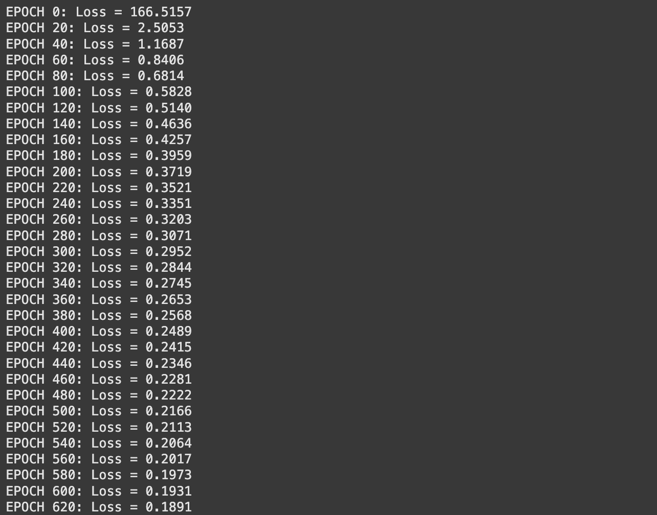

Then we can visualize the output of the neural network’s prediction vs the actual function.

import matplotlib.pyplot as plt

# Reshape predictions to grid format for visualization
Z_pred = model.predict(inputs) * outputs_std + outputs_mean
Z_pred = Z_pred.reshape(X.shape)

# Plot comparison of the true function and the model predictions
fig, axes = plt.subplots(1, 2, figsize=(14, 6))

# Plot the true function
axes[0].contourf(X, Y, Z, cmap='viridis')
axes[0].set_title("True Function")
axes[0].set_xlabel("X-axis")
axes[0].set_ylabel("Y-axis")
axes[0].colorbar = plt.colorbar(axes[0].contourf(X, Y, Z, cmap='viridis'), ax=axes[0], label="Function Value")

# Plot the predicted function
axes[1].contourf(X, Y, Z_pred, cmap='plasma')
axes[1].set_title("NN Predicted Function")
axes[1].set_xlabel("X-axis")
axes[1].set_ylabel("Y-axis")
axes[1].colorbar = plt.colorbar(axes[1].contourf(X, Y, Z_pred, cmap='plasma'), ax=axes[1], label="Function Value")

plt.tight_layout()
plt.show()

This did an ok job, but not as great as we might like. This is where a lot of data scientists spend their time, and there are a ton of approaches to making a neural network fit a certain problem better. Some obvious ones are:

• use more data
• play around with the learning rate
• train for more epochs
• change the structure of the model

It’s pretty easy for us to crank up the amount of data we’re training on. Let’s see where that leads us. Here I’m sampling our dataset 10,000 times, which is 10x more training samples than our previous dataset.

And then I trained the model just like before, except this time it took a lot longer because each epoch now analyses 10,000 samples rather than 1,000.

# Define the architecture: [input_dim, hidden1, ..., output_dim]
architecture = [2, 64, 64, 64, 1]  # Two inputs, two hidden layers, one output
model = SimpleNN(architecture)

# Train the model
model.train(inputs, outputs, epochs=2000, lr=0.001)

I then rendered the output of this model, the same way I did before, but it didn’t really look like the output got much better.

Looking back at the loss output from training, it seems like the loss is still steadily declining. Maybe I just need to train for longer. Let’s try that.

# Define the architecture: [input_dim, hidden1, ..., output_dim]
architecture = [2, 64, 64, 64, 1]  # Two inputs, two hidden layers, one output
model = SimpleNN(architecture)

# Train the model
model.train(inputs, outputs, epochs=4000, lr=0.001)

The results seem to be a bit better, but they aren’t’ amazing.

I’ll spare you the details. I ran this a few times, and I got some decent results, but never anything 1 to 1. I’ll be covering some more advanced approaches data scientists use, like annealing and dropout, in future articles which will result in a more consistent and better output. Still, though, we made a neural network from scratch and trained it to do something, and it did a decent job! Pretty neat!

Conclusion

In this article we avoided calculus like the plague while simultaneously forging an understanding of Neural Networks. We explored their theory, a little bit about the math, the idea of back propagation, and then implemented a neural network from scratch. We then applied a neural network to a toy problem, and explored some of the simple ideas data scientists employ to actually train neural networks to be good at things.

In future articles we’ll explore a few more advanced approaches to Neural Networks, so stay tuned! For now, you might be interested in a more thorough analysis of Gradients, the fundamental math behind back propagation.

What Are Gradients, and Why Do They Explode?

You might also be interested in this article, which covers training a neural network using more conventional Data Science tools like PyTorch.

AI for the Absolute Novice – Intuitively and Exhaustively Explained

Join Intuitively and Exhaustively Explained

At IAEE you can find:

• Long form content, like the article you just read
• Conceptual breakdowns of some of the most cutting-edge AI topics
• By-Hand walkthroughs of critical mathematical operations in AI
• Practical tutorials and explainers

The post Neural Networks – Intuitively and Exhaustively Explained appeared first on Towards Data Science.