DeepSeek-V3 Explained 1: Multi-head Latent Attention

Key architecture innovation behind DeepSeek-V2 and DeepSeek-V3 for faster inference

This is the first article of our new series “DeepSeek-V3 Explained”, where we will try to demystify DeepSeek-V3 [1, 2], the latest model open-sourced by DeepSeek.

In this series, we aim to cover two major topics:

• Major architecture innovations in DeepSeek-V3, including MLA (Multi-head Latent Attention) [3], DeepSeekMoE [4], auxiliary-loss-free load balancing [5], and multi-token prediction training.
• Training of DeepSeek-V3, including pre-training, finetuning and RL alignment phases.

This article mainly focuses on Multi-head Latent Attention, which was first proposed in the development of DeepSeek-V2 and then used in DeepSeek-V3 as well.

Table of contents:

• Background: we start from the standard MHA, explain why we need Key-Value cache at inference stage, how MQA and GQA try to optimize it, and how RoPE works, etc.
• Multi-head Latent Attention: An in-depth introduction to MLA, including its motivations, why decoupled RoPE is needed, and its performance.
• References.

Background

To better understand MLA and also make this article self-contained, we will revisit several related concepts in this section before diving into the details of MLA.

MHA in Decoder-only Transformers

Note that MLA is developed to speedup inference speed in autoregressive text generation, so the MHA we are talking about under this context is for decoder-only Transformer.

The figure below compares three Transformer architectures used for decoding, where (a) shows both the encoder and decoder proposed in the original “Attention is All You Need” paper. Its decoder part is then simplified by [6], leading to a decoder-only Transformer model shown in (b), which is later used in many generation models like GPT [8].

Nowadays, LLMs are more commonly to choose the structure shown in (c) for more stable training, with normalization applied on the input rather then output, and LayerNorm upgraded to RMS Norm. This will serve as the baseline architecture we will discuss in this article.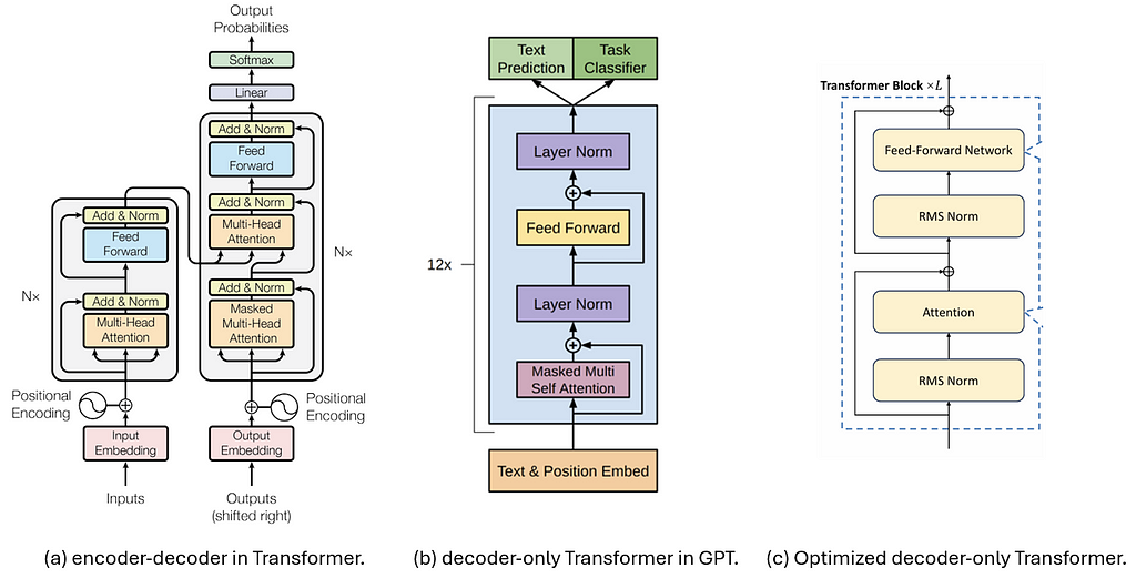

Within this context, MHA calculation largely follows the process in [6], as shown in the figure below: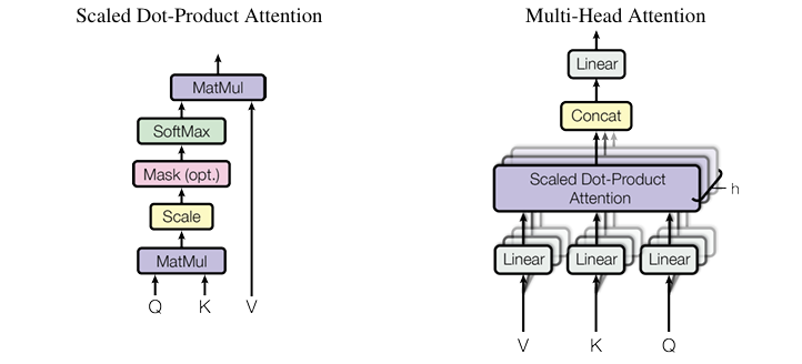

Assume we have n_h attention heads, and the dimension for each attention head is represented as d_h, so that the concatenated dimension will be (h_n · d_h).

Given a model with l layers, if we denote the input for the t-th token in that layer as h_t with dimension d, we need to map the dimension of h_t from d to (h_n · d_h) using the linear mapping matrices.

More formally, we have (equations from [3]):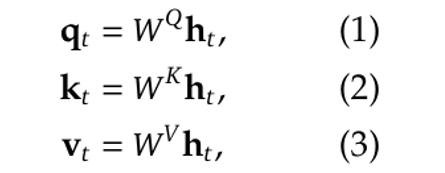

where W^Q, W^K and W^V are the linear mapping matrices:

After such mapping, q_t, k_t and v_t will be split into n_h heads to calculate the scaled dot-product attention:

where W^O is another projection matrix to map the dimension inversely from (h_n · d_h) to d:

Note that the process described by Eqn.(1) to (8) above is just for a single token. During inference, we need to repeat this process for each newly generated token, which involves a lot of repeated calculation. This leads to a technique called Key-Value cache.

Key-Value Cache

As suggested by its name, Key-Value cache is a technique designed to speedup the autoregressive process by caching and reusing the previous keys and values, rather than re-computing them at each decoding step.

Note that KV cache is typically used only during the inference stage, since in training we still need to process the entire input sequence in parallel.

KV cache is commonly implemented as a rolling buffer. At each decoding step, only the new query Q is computed, while the K and V stored in the cache will be reused, so that the attention will be computed using the new Q and reused K, V. Meanwhile, the new token’s K and V will also be appended to the cache for later use.

However, the speedup achieved by KV cache comes at a cost of memory, since KV cache often scales with batch size × sequence length × hidden size × number of heads, leading to a memory bottleneck when we have larger batch size or longer sequences.

That further leads to two techniques aiming at addressing this limitation: Multi-Query Attention and Grouped-Query Attention.

Multi-Query Attention (MQA) vs Grouped-Query Attention (GQA)

The figure below shows the comparison between the original MHA, Grouped-Query Attention (GQA) [10] and Multi-Query Attention (MQA) [9].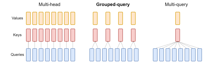

The basic idea of MQA is to share a single key and a single value head across all query heads, which can significantly reduce memory usage but will also impact the accuracy of attention.

GQA can be seen as an interpolating method between MHA and MQA, where a single pair of key and value heads will be shared only by a group of query heads, not all queries. But still this will lead to inferior results compared to MHA.

In the later sections, we will see how MLA manages to seek a balance between memory efficiency and modeling accuracy.

RoPE (Rotary Positional Embeddings)

One last piece of background we need to mention is RoPE [11], which encodes positional information directly into the attention mechanism by rotating the query and key vectors in multi-head attention using sinusoidal functions.

More specifically, RoPE applies a position-dependent rotation matrix to the query and key vectors at each token, and uses sine and cosine functions for its basis but applies them in a unique way to achieve rotation.

To see what makes it position-dependent, consider a toy embedding vector with only 4 elements, i.e., (x_1, x_2, x_3, x_4).

To apply RoPE, we firstly group consecutive dimensions into pairs:

• (x_1, x_2) -> position 1
• (x_3, x_4) -> position 2

Then, we apply a rotation matrix to rotate each pair: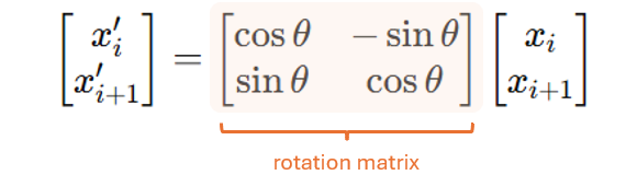

where θ = θ(p) = p ⋅ θ_0​, and θ_0​ is a base frequency. In our 4-d toy example, this means that (x_1, x_2) will be rotated by θ_0​, and (x_3, x_4) will be rotated by 2 ⋅ θ_0.

This is why we call this rotation matrix as position-dependent: at each position (or each pair), we will apply a different rotation matrix where the rotation angle is determined by position.

RoPE is widely used in modern LLMs due to its efficiency in encoding long sequences, but as we can see from the above formula, it is position-sensitive to both Q and K, making it incompatible with MLA in some ways.

Multi-head Latent Attention

Finally we can move on to the MLA part. In this section we will first layout the high-level idea of MLA, and then dive deeper into why it needs to modify RoPE. Finally, we present the detailed algorithm of MLA as well as it performance.

MLA: High-level Idea

The basic idea of MLA is to compress the attention input h_t into a low-dimensional latent vector with dimension d_c, where d_c is much lower than the original (h_n · d_h). Later when we need to calculate attention, we can map this latent vector back to the high-dimensional space to recover the keys and values. As a result, only the latent vector needs to be stored, leading to significant memory reduction.

This process can be more formally described with the following equations, where c^{KV}_t is the latent vector, W^{DKV} is the compressing matrix that maps h_t’s dimension from (h_n · d_h) to d_c (here D in the superscript stands for “down-projection”, meaning compressing the dimension), while W^{UK} and W^{UV} are both up-projection matrices that map the shared latent vector back to the high-dimensional space.

Similarly, we can also map the queries into a latent, low-dimensional vector and then map it back to the original, high-dimensional space: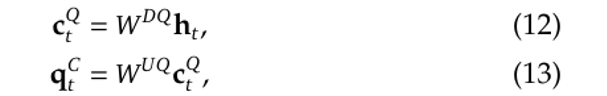

Why Decoupled RoPE is Needed

As we mentioned before, RoPE is a common choice for training generation models to handle long sequences. If we directly apply the above MLA strategy, that will be incompatible with RoPE.

To see this more clearly, consider what happens when we calculate attention using Eqn. (7): when we multiply the transposed q with k, the matrices W^Q and W^{UK} will appear in the middle, and their combination equivalents to a single mapping dimension from d_c to d.

In the original paper [3], the authors describe this as W^{UK} can be “absorbed” into W^Q, as a result we do not need to store W^{UK} in the cache, further reducing memory usage.

However, this will not be the case when we take the rotation matrix in Figure (4) into consideration, as RoPE will apply a rotation matrix on the left of W^{UK}, and this rotation matrix will end up in between the transposed W^Q and W^{UK}.

As we have explained in the background part, this rotation matrix is position-dependent, meaning the rotation matrix for each position is different. As a result, W^{UK} can no longer be absorbed by W^Q.

To address this conflict, the authors propose what they call “a decoupled RoPE”, by introducing additional query vectors along with a shared key vector, and use these additional vectors in the RoPE process only, while keeping the original keys kind of isolated with the rotation matrix.

The entire process of MLA can be summarized as below (equation numbers reused from Appendix C in [3]):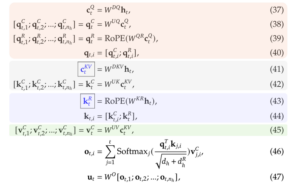

where

• Eqn. (37) to (40) describe how to process query tokens.
• Eqn. (41) and (42) describe how to process key tokens.
• Eqn. (43) and (44) describe how to use the additional shared key for RoPE, be aware that the output of (42) is not involved in RoPE.
• Eqn. (45) describes how to process value tokens.

During this process, only the blue variables with boxes need to be cached. This process can be illustrated more clearly with the flowchart blow: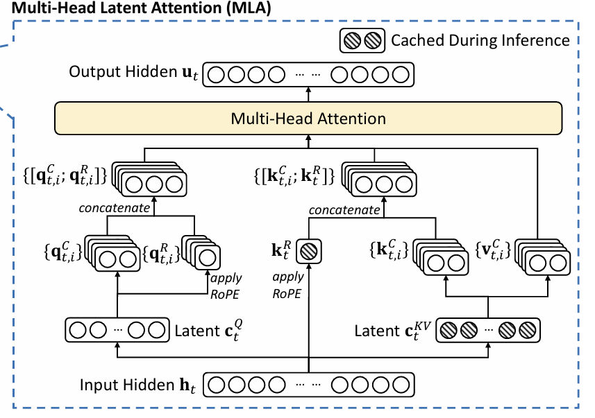

Performance of MLA

The table below compares the number of elements needed for KV cache (per token) as well as the modeling capacity between MHA, GQA, MQA and MLA, demonstrating that MLA could indeed achieve a better balance between memory efficiency vs. modeling capacity.

Interestingly, the modeling capacity for MLA even surpass that of the original MHA.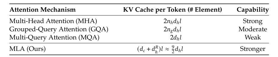

More specifically, the table below shows the performance of MHA, GQA and MQA on 7B models, where MHA significantly outperforms both MQA and GQA.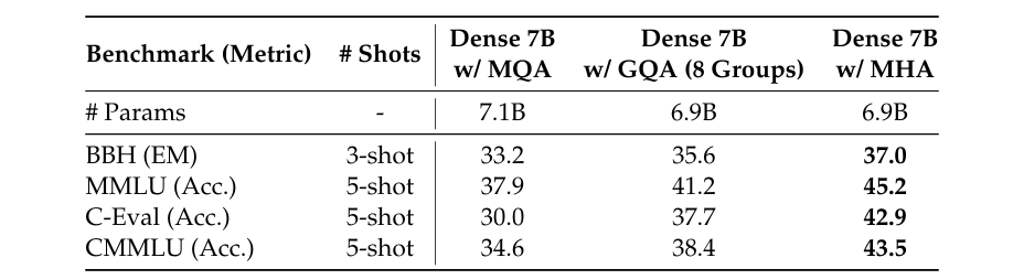

The authors of [3] also conduct analysis between MHA vs. MLA, and results are summarized in the table below, where MLA achieves better results overall.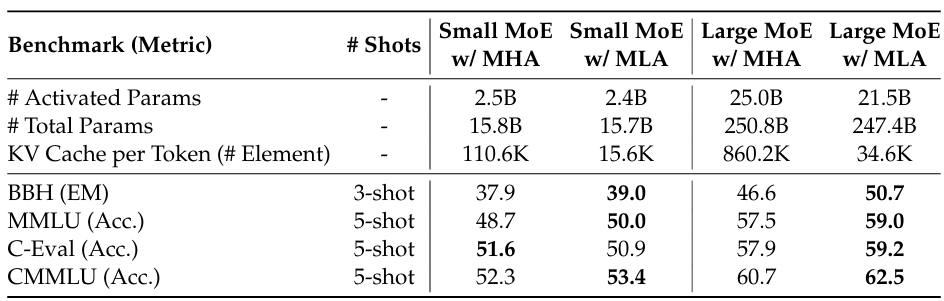

References

• [1] DeepSeek
• [2] DeepSeek-V3 Technical Report
• [3] DeepSeek-V2: A Strong, Economical, and Efficient Mixture-of-Experts Language Model
• [4] DeepSeekMoE: Towards Ultimate Expert Specialization in Mixture-of-Experts Language Models
• [5] Auxiliary-Loss-Free Load Balancing Strategy for Mixture-of-Experts
• [6] Attention Is All You Need
• [7] Generating Wikipedia by Summarizing Long Sequences
• [8] Improving Language Understanding by Generative Pre-Training
• [9] Fast Transformer Decoding: One Write-Head is All You Need
• [10] GQA: Training Generalized Multi-Query Transformer Models from Multi-Head Checkpoints
• [11] RoFormer: Enhanced Transformer with Rotary Position Embedding

DeepSeek-V3 Explained 1: Multi-head Latent Attention was originally published in Towards Data Science on Medium, where people are continuing the conversation by highlighting and responding to this story.